library(tidyverse)
library(srvyr)
library(srvyrexploR)03 - Descriptive Analysis
Slides
Your Turn
Set-up
Load necessary packages
Load in data and preview it
glimpse(recs_2020)Rows: 18,496
Columns: 100
$ DOEID <dbl> 100001, 100002, 100003, 100004, 100005, 100006, 10000…
$ ClimateRegion_BA <fct> Mixed-Dry, Mixed-Humid, Mixed-Dry, Mixed-Humid, Mixed…
$ Urbanicity <fct> Urban Area, Urban Area, Urban Area, Urban Area, Urban…
$ Region <fct> West, South, West, South, Northeast, South, South, So…
$ REGIONC <chr> "WEST", "SOUTH", "WEST", "SOUTH", "NORTHEAST", "SOUTH…
$ Division <fct> Mountain South, West South Central, Mountain South, S…
$ STATE_FIPS <chr> "35", "05", "35", "45", "34", "48", "40", "28", "11",…
$ state_postal <fct> NM, AR, NM, SC, NJ, TX, OK, MS, DC, AZ, CA, TX, LA, M…
$ state_name <fct> New Mexico, Arkansas, New Mexico, South Carolina, New…
$ HDD65 <dbl> 3844, 3766, 3819, 2614, 4219, 901, 3148, 1825, 4233, …
$ CDD65 <dbl> 1679, 1458, 1696, 1718, 1363, 3558, 2128, 2374, 1159,…
$ HDD30YR <dbl> 4451, 4429, 4500, 3229, 4896, 1150, 3564, 2660, 4404,…
$ CDD30YR <dbl> 1027, 1305, 1010, 1653, 1059, 3588, 2043, 2164, 1407,…
$ HousingUnitType <fct> Single-family detached, Apartment: 5 or more units, A…
$ YearMade <ord> 1970-1979, 1980-1989, 1960-1969, 1980-1989, 1960-1969…
$ TOTSQFT_EN <dbl> 2100, 590, 900, 2100, 800, 4520, 2100, 900, 750, 760,…
$ TOTHSQFT <dbl> 2100, 590, 900, 2100, 800, 3010, 1200, 900, 750, 760,…
$ TOTCSQFT <dbl> 2100, 590, 900, 2100, 800, 3010, 1200, 0, 500, 760, 1…
$ SpaceHeatingUsed <lgl> TRUE, TRUE, TRUE, TRUE, TRUE, TRUE, TRUE, TRUE, TRUE,…
$ ACUsed <lgl> TRUE, TRUE, TRUE, TRUE, TRUE, TRUE, TRUE, FALSE, TRUE…
$ HeatingBehavior <fct> Set one temp and leave it, Turn on or off as needed, …
$ WinterTempDay <dbl> 70, 70, 69, 68, 68, 76, 74, 70, 68, 70, 72, 74, 74, 7…
$ WinterTempAway <dbl> 70, 65, 68, 68, 68, 76, 65, 70, 60, 70, 70, 74, 74, 7…
$ WinterTempNight <dbl> 68, 65, 67, 68, 68, 68, 74, 68, 62, 68, 72, 74, 74, 6…
$ ACBehavior <fct> Set one temp and leave it, Turn on or off as needed, …
$ SummerTempDay <dbl> 71, 68, 70, 72, 72, 69, 68, NA, 72, 74, 77, 77, 74, 6…
$ SummerTempAway <dbl> 71, 68, 68, 72, 72, 74, 70, NA, 76, 74, 77, 77, 74, 6…
$ SummerTempNight <dbl> 71, 68, 68, 72, 72, 68, 70, NA, 68, 72, 77, 77, 74, 6…
$ NWEIGHT <dbl> 3284.104, 9007.387, 5669.002, 5294.239, 9935.465, 724…
$ NWEIGHT1 <dbl> 3273.053, 9019.564, 5793.353, 5361.146, 10047.545, 73…
$ NWEIGHT2 <dbl> 3349.139, 9081.268, 5913.554, 5361.706, 10261.682, 74…
$ NWEIGHT3 <dbl> 3344.876, 9020.409, 5762.743, 5371.011, 10036.522, 73…
$ NWEIGHT4 <dbl> 3437.284, 9213.074, 5870.261, 5392.846, 9960.953, 742…
$ NWEIGHT5 <dbl> 3415.582, 9117.337, 5720.669, 5327.617, 10107.863, 73…
$ NWEIGHT6 <dbl> 3354.813, 9178.697, 5662.939, 5353.957, 10298.428, 74…
$ NWEIGHT7 <dbl> 3372.342, 9095.936, 5699.536, 5325.316, 10064.709, 73…
$ NWEIGHT8 <dbl> 3364.035, 8920.480, 5704.027, 5375.732, 10096.509, 73…
$ NWEIGHT9 <dbl> 3361.912, 9188.981, 5667.670, 5391.379, 10321.424, 73…
$ NWEIGHT10 <dbl> 3301.569, 9060.009, 5793.325, 5500.628, 9943.547, 731…
$ NWEIGHT11 <dbl> 3211.291, 9127.404, 5806.321, 5427.320, 10266.593, 73…
$ NWEIGHT12 <dbl> 3500.495, 9264.304, 5650.394, 5384.442, 10127.061, 73…
$ NWEIGHT13 <dbl> 3313.754, 9222.011, 5648.461, 5302.085, 10240.975, 72…
$ NWEIGHT14 <dbl> 3359.110, 9199.014, 5828.712, 5362.226, 9871.649, 740…
$ NWEIGHT15 <dbl> 3423.682, 9143.214, 5641.887, 5383.136, 10275.303, 74…
$ NWEIGHT16 <dbl> 3383.601, 9042.382, 5717.847, 5380.916, 9921.199, 738…
$ NWEIGHT17 <dbl> 3312.112, 9416.815, 5968.713, 5418.300, 10311.952, 73…
$ NWEIGHT18 <dbl> 3324.383, 9162.681, 5828.370, 5356.271, 10004.213, 74…
$ NWEIGHT19 <dbl> 3366.644, 9191.950, 5814.049, 5343.187, 10437.297, 75…
$ NWEIGHT20 <dbl> 3326.643, 9091.550, 5697.447, 5360.409, 10100.730, 73…
$ NWEIGHT21 <dbl> 3339.910, 0.000, 5686.769, 5336.323, 9981.635, 7427.5…
$ NWEIGHT22 <dbl> 3292.197, 9097.877, 5738.946, 5389.830, 10000.278, 73…
$ NWEIGHT23 <dbl> 3277.697, 9319.896, 5944.649, 5397.093, 10179.723, 71…
$ NWEIGHT24 <dbl> 3340.406, 9080.729, 5819.996, 5448.089, 9825.700, 746…
$ NWEIGHT25 <dbl> 3386.445, 9406.487, 5823.075, 5382.111, 10149.386, 72…
$ NWEIGHT26 <dbl> 3300.574, 9255.867, 5650.188, 5386.710, 0.000, 7309.1…
$ NWEIGHT27 <dbl> 3311.546, 9318.078, 5862.116, 5351.082, 10140.604, 72…
$ NWEIGHT28 <dbl> 3347.637, 9154.189, 5706.909, 5371.439, 9948.403, 750…
$ NWEIGHT29 <dbl> 3355.638, 9371.695, 5618.615, 5361.572, 10064.708, 73…
$ NWEIGHT30 <dbl> 3322.423, 9137.197, 5795.544, 5381.218, 10082.927, 73…
$ NWEIGHT31 <dbl> 3255.840, 9233.363, 5994.544, 5319.728, 10132.977, 73…
$ NWEIGHT32 <dbl> 3317.937, 9114.608, 0.000, 5338.558, 9978.370, 7302.5…
$ NWEIGHT33 <dbl> 3401.811, 9176.872, 5637.872, 0.000, 10213.075, 7326.…
$ NWEIGHT34 <dbl> 3363.592, 9191.207, 5619.040, 5379.523, 9964.337, 724…
$ NWEIGHT35 <dbl> 3303.528, 9100.344, 5652.289, 5363.277, 10070.847, 0.…
$ NWEIGHT36 <dbl> 3333.027, 9071.530, 5834.171, 5476.866, 9987.947, 735…
$ NWEIGHT37 <dbl> 3389.869, 9263.141, 5712.198, 5386.333, 10120.314, 73…
$ NWEIGHT38 <dbl> 3381.503, 9077.901, 5765.422, 5326.402, 10023.636, 73…
$ NWEIGHT39 <dbl> 3328.893, 9011.009, 5887.338, 5420.540, 10023.919, 73…
$ NWEIGHT40 <dbl> 3292.829, 9166.222, 5649.809, 5370.189, 10184.527, 73…
$ NWEIGHT41 <dbl> 3295.089, 9091.334, 5957.748, 5339.323, 10069.084, 73…
$ NWEIGHT42 <dbl> 3413.593, 9193.664, 5592.619, 5328.788, 9958.721, 743…
$ NWEIGHT43 <dbl> 3263.710, 9215.337, 6035.472, 5409.435, 10352.485, 73…
$ NWEIGHT44 <dbl> 3342.446, 9048.092, 5732.384, 5416.488, 10091.807, 74…
$ NWEIGHT45 <dbl> 3275.274, 9258.580, 5876.696, 5453.165, 10227.529, 74…
$ NWEIGHT46 <dbl> 3364.248, 9170.518, 5653.511, 5449.444, 10069.384, 73…
$ NWEIGHT47 <dbl> 3336.066, 9260.064, 5763.458, 5375.551, 9995.686, 732…
$ NWEIGHT48 <dbl> 3329.151, 9105.220, 5928.968, 5407.834, 10197.608, 73…
$ NWEIGHT49 <dbl> 3348.061, 9116.891, 5772.333, 5399.779, 10093.620, 74…
$ NWEIGHT50 <dbl> 3357.231, 9261.127, 5785.452, 5359.408, 10196.251, 73…
$ NWEIGHT51 <dbl> 3335.188, 8955.288, 5635.561, 5447.619, 10017.094, 73…
$ NWEIGHT52 <dbl> 3240.132, 9000.296, 5944.330, 5344.453, 9954.142, 749…
$ NWEIGHT53 <dbl> 3429.728, 9290.375, 5683.500, 5437.803, 10050.961, 74…
$ NWEIGHT54 <dbl> 3294.084, 9199.326, 5735.631, 5377.898, 10018.844, 72…
$ NWEIGHT55 <dbl> 3397.713, 8958.782, 5674.564, 5357.470, 10309.728, 75…
$ NWEIGHT56 <dbl> 3292.610, 9232.597, 5660.854, 5421.025, 10142.763, 73…
$ NWEIGHT57 <dbl> 0.000, 9140.427, 5917.193, 5365.230, 10176.828, 7383.…
$ NWEIGHT58 <dbl> 3369.768, 9306.997, 5571.015, 5402.057, 10043.143, 75…
$ NWEIGHT59 <dbl> 3358.163, 9061.782, 5887.092, 5402.772, 10247.911, 73…
$ NWEIGHT60 <dbl> 3404.031, 8957.915, 5837.846, 5350.860, 10110.301, 75…
$ BTUEL <dbl> 42723.28, 17889.29, 8146.63, 31646.53, 20027.42, 4896…
$ DOLLAREL <dbl> 1955.06, 713.27, 334.51, 1424.86, 1087.00, 1895.66, 1…
$ BTUNG <dbl> 101924.43, 10145.32, 22603.08, 55118.66, 39099.51, 36…
$ DOLLARNG <dbl> 701.8300, 261.7348, 188.1400, 636.9100, 376.0400, 439…
$ BTULP <dbl> 0.00, 0.00, 0.00, 0.00, 0.00, 0.00, 0.00, 0.00, 0.00,…
$ DOLLARLP <dbl> 0.00, 0.00, 0.00, 0.00, 0.00, 0.00, 0.00, 0.00, 0.00,…
$ BTUFO <dbl> 0.00, 0.00, 0.00, 0.00, 0.00, 0.00, 0.00, 0.00, 0.00,…
$ DOLLARFO <dbl> 0.00, 0.00, 0.00, 0.00, 0.00, 0.00, 0.00, 0.00, 0.00,…
$ BTUWOOD <dbl> 0, 0, 0, 0, 0, 3000, 0, 0, 0, 0, 0, 0, 0, 0, 0, 0, 0,…
$ TOTALBTU <dbl> 144647.71, 28034.61, 30749.71, 86765.19, 59126.93, 85…
$ TOTALDOL <dbl> 2656.8900, 975.0048, 522.6500, 2061.7700, 1463.0400, …glimpse(anes_2020)Rows: 7,453
Columns: 65
$ V200001 <dbl> 200015, 200022, 200039, 200046, 200053, 200060…
$ CaseID <dbl> 200015, 200022, 200039, 200046, 200053, 200060…
$ V200002 <hvn_lbll> 3, 3, 3, 3, 3, 3, 3, 3, 3, 3, 3, 3, 3, 3,…
$ InterviewMode <fct> Web, Web, Web, Web, Web, Web, Web, Web, Web, W…
$ V200010b <dbl> 1.0057375, 1.1634731, 0.7686811, 0.5210195, 0.…
$ Weight <dbl> 1.0057375, 1.1634731, 0.7686811, 0.5210195, 0.…
$ V200010c <dbl> 2, 2, 1, 2, 1, 2, 1, 2, 2, 2, 1, 1, 2, 2, 2, 2…
$ VarUnit <fct> 2, 2, 1, 2, 1, 2, 1, 2, 2, 2, 1, 1, 2, 2, 2, 2…
$ V200010d <dbl> 9, 26, 41, 29, 23, 37, 7, 37, 32, 41, 22, 7, 3…
$ Stratum <fct> 9, 26, 41, 29, 23, 37, 7, 37, 32, 41, 22, 7, 3…
$ V201006 <hvn_lbll> 2, 3, 2, 3, 2, 1, 2, 3, 2, 2, 2, 2, 2, 1,…
$ CampaignInterest <fct> Somewhat interested, Not much interested, Some…
$ V201023 <hvn_lbll> -1, -1, -1, -1, -1, -1, -1, -1, 1, -1, -1…
$ EarlyVote2020 <fct> NA, NA, NA, NA, NA, NA, NA, NA, Yes, NA, NA, N…
$ V201024 <hvn_lbll> -1, -1, -1, -1, -1, -1, -1, -1, 2, -1, -1…
$ V201025x <hvn_lbll> 3, 3, 3, 3, 3, 3, 3, 2, 4, 3, 3, 3, 2, 4,…
$ V201028 <hvn_lbll> -1, -1, -1, -1, -1, -1, -1, -1, 1, -1, -1…
$ V201029 <hvn_lbll> -1, -1, -1, -1, -1, -1, -1, -1, 1, -1, -1…
$ V201101 <hvn_lbll> -1, -1, -1, -1, -1, -1, -1, -1, 1, 1, 2, …
$ V201102 <hvn_lbll> 1, 1, 1, 1, 1, 2, 1, 2, -1, -1, -1, 1, 2,…
$ VotedPres2016 <fct> Yes, Yes, Yes, Yes, Yes, No, Yes, No, Yes, Yes…
$ V201103 <hvn_lbll> 2, 5, 1, 1, 2, -1, 5, -1, 1, 1, -1, 1, -1…
$ VotedPres2016_selection <fct> Trump, Other, Clinton, Clinton, Trump, NA, Oth…
$ V201228 <hvn_lbll> 2, 5, 3, 2, 3, 3, 2, 2, 3, 1, 1, 1, 2, 1,…
$ V201229 <hvn_lbll> 1, -1, -1, 2, -1, -1, 2, 2, -1, 2, 1, 2, …
$ V201230 <hvn_lbll> -1, 2, 3, -1, 2, 3, -1, -1, 2, -1, -1, -1…
$ V201231x <hvn_lbll> 7, 4, 3, 6, 4, 3, 6, 6, 4, 2, 1, 2, 7, 2,…
$ PartyID <fct> Strong republican, Independent, Independent-de…
$ V201233 <hvn_lbll> 5, 5, 4, 3, 5, 4, 4, 1, 3, 3, 2, 3, 4, 5,…
$ TrustGovernment <fct> Never, Never, Some of the time, About half the…
$ V201237 <hvn_lbll> 3, 4, 4, 2, 4, 2, 4, 1, 3, 2, 4, 3, 4, 3,…
$ TrustPeople <fct> About half the time, Some of the time, Some of…
$ V201507x <hvn_lbll> 46, 37, 40, 41, 72, 71, 37, 45, 70, 43, 3…
$ Age <dbl> 46, 37, 40, 41, 72, 71, 37, 45, 70, 43, 37, 55…
$ AgeGroup <fct> 40-49, 30-39, 40-49, 40-49, 70 or older, 70 or…
$ V201510 <hvn_lbll> 6, 3, 2, 4, 8, 3, 4, 2, 2, 4, 2, 2, 2, 7,…
$ Education <fct> Bachelor's, Post HS, High school, Post HS, Gra…
$ V201546 <hvn_lbll> 1, 2, 2, 2, 2, 2, 2, 2, 2, 1, 1, 2, 2, 2,…
$ V201547a <hvn_lbll> -3, -3, -3, -3, -3, -3, -3, -3, -3, -3, -…
$ V201547b <hvn_lbll> -3, -3, -3, -3, -3, -3, -3, -3, -3, -3, -…
$ V201547c <hvn_lbll> -3, -3, -3, -3, -3, -3, -3, -3, -3, -3, -…
$ V201547d <hvn_lbll> -3, -3, -3, -3, -3, -3, -3, -3, -3, -3, -…
$ V201547e <hvn_lbll> -3, -3, -3, -3, -3, -3, -3, -3, -3, -3, -…
$ V201547z <hvn_lbll> -3, -3, -3, -3, -3, -3, -3, -3, -3, -3, -…
$ V201549x <hvn_lbll> 3, 4, 1, 4, 5, 1, 1, 1, 1, 3, 3, 1, 1, 4,…
$ RaceEth <fct> "Hispanic", "Asian, NH/PI", "White", "Asian, N…
$ V201600 <hvn_lbll> 1, 2, 2, 1, 1, 2, 2, 2, 2, 1, 2, 1, 2, 1,…
$ Gender <fct> Male, Female, Female, Male, Male, Female, Fema…
$ V201607 <hvn_lbll> -3, -3, -3, -3, -3, -3, -3, -3, -3, -3, -…
$ V201610 <hvn_lbll> -3, -3, -3, -3, -3, -3, -3, -3, -3, -3, -…
$ V201611 <hvn_lbll> -3, -3, -3, -3, -3, -3, -3, -3, -3, -3, -…
$ V201613 <hvn_lbll> -3, -3, -3, -3, -3, -3, -3, -3, -3, -3, -…
$ V201615 <hvn_lbll> -3, -3, -3, -3, -3, -3, -3, -3, -3, -3, -…
$ V201616 <hvn_lbll> -3, -3, -3, -3, -3, -3, -3, -3, -3, -3, -…
$ V201617x <hvn_lbll> 21, 13, 17, 7, 22, 3, 4, 3, 10, 11, 9, 18…
$ Income <fct> "$175,000-249,999", "$70,000-74,999", "$100,00…
$ Income7 <fct> $125k or more, $60k to < 80k, $100k to < 125k,…
$ V202051 <hvn_lbll> -1, -1, -1, -1, -1, -1, -1, 1, -1, -1, -1…
$ V202066 <hvn_lbll> 1, 4, 4, 4, 4, 4, 4, 1, -1, 4, 4, 4, 4, -…
$ V202072 <hvn_lbll> -1, 1, 1, 1, 1, 1, 1, -1, -1, 1, 1, 1, 1,…
$ VotedPres2020 <fct> NA, Yes, Yes, Yes, Yes, Yes, Yes, NA, Yes, Yes…
$ V202073 <hvn_lbll> -1, 3, 1, 1, 2, 1, 2, -1, -1, 1, 1, 1, 2,…
$ V202109x <hvn_lbll> 0, 1, 1, 1, 1, 1, 1, 0, 1, 1, 1, 1, 1, 1,…
$ V202110x <hvn_lbll> -1, 3, 1, 1, 2, 1, 2, -1, 1, 1, 1, 1, 2, …
$ VotedPres2020_selection <fct> NA, Other, Biden, Biden, Trump, Biden, Trump, …Find codebooks here:
Create design objects for usage
anes_des <- anes_2020 %>%
  mutate(Weight = V200010b / sum(V200010b) * 231034125) %>%
  as_survey_design(
    weights = Weight,
    strata = V200010d,
    ids = V200010c,
    nest = TRUE
  )

recs_des <- recs_2020 %>%
  as_survey_rep(
    weights = NWEIGHT,
    repweights = NWEIGHT1:NWEIGHT60,
    type = "JK1",
    scale = 59 / 60,
    mse = TRUE
  )
Exercises - Part 1
- How many females have a graduate degree (according to the ANES data)?
# Hint: The variables `Gender` and `Education` will be useful.- What percentage of people identify as “Strong Democrat”?
# Hint: The variable `PartyID` indicates someone’s party affiliation.- What percentage of people who voted in the 2020 election identify as “Strong Republican”?
# Hint: The variable `VotedPres2020` indicates whether someone voted in 2020.- What percentage of people voted in both the 2016 election and the 2020 election? Include the logit confidence interval.
# Hint: The variable VotedPres2016 indicates whether someone voted in 2016.- Advanced bonus exercise What percentage of people used air-conditioning (A/C) in each state according to the RECS data? Extra bonus: Make a plot or map of this data by state - the usmap package may be useful.
# Hint: The variable `state_postal` indicates the state and `ACUsed` indicates whether the household used A/CExercises - Part 2
- What is the design effect for the proportion of people who voted early?
# Hint: The variable `EarlyVote2020` indicates whether someone voted early in 2020.- What is the median temperature people set their thermostats to at night during the winter (using the RECS data)?
# Hint: The variable `WinterTempNight` indicates the temperature that people set their thermostat to in the winter at night.- People sometimes set their temperature differently over different seasons and during the day. What median temperatures do people set their thermostats to in the summer and winter, both during the day and at night? Include confidence intervals.
# Hint: Use the variables `WinterTempDay`, `WinterTempNight`, `SummerTempDay`, and `SummerTempNight.`- What is the correlation between the temperature that people set their temperature at during the night and during the day in the summer?
# Hint: use the variables `SummerTempNight` and `SummerTempDay`- What is the 1st, 2nd, and 3rd quartile of money spent on energy by Building America (BA) climate zone? Include the national estimates as well.
# Hint: `TOTALDOL` indicates the total amount spent on all fuel, and `ClimateRegion_BA` indicates the BA climate zones.- Advanced bonus exercise What is the average money spent on energy per square foot by state? Extra bonus: Make a plot or map of this data by state
# Hint: The variable `state_postal` indicates the state, `TOTALDOL` is the amount of money spent on energy, and `TOTSQFT_EN` is the square footageSolutions
See the solutions
Exercises - Part 1
- How many females have a graduate degree (according to the ANES data)?
Show code
anes_des %>%
  survey_count(Gender, Education) %>%
  filter(Gender == "Female", Education == "Graduate")
# A tibble: 1 × 4
Gender Education n n_se
<fct> <fct> <dbl> <dbl>
1 Female Graduate 15072196. 837872.- What percentage of people identify as “Strong Democrat”?
Show code
anes_des %>%
  group_by(PartyID) %>%
  summarize(
    p = survey_prop()
  ) %>%
  filter(PartyID == "Strong democrat")
When `proportion` is unspecified, `survey_prop()` now defaults to `proportion = TRUE`.
ℹ This should improve confidence interval coverage.
This message is displayed once per session.# A tibble: 1 × 3
PartyID p p_se
<fct> <dbl> <dbl>
1 Strong democrat 0.219 0.00646- What percentage of people who voted in the 2020 election identify as “Strong Republican”?
Show code
anes_des %>%
  filter(VotedPres2020 == "Yes") %>%
  group_by(PartyID) %>%
  summarize(
    p = survey_prop()
  ) %>%
  filter(PartyID == "Strong republican")
# A tibble: 1 × 3
PartyID p p_se
<fct> <dbl> <dbl>
1 Strong republican 0.228 0.00824- What percentage of people voted in both the 2016 election and the 2020 election? Include the logit confidence interval.
Show code
anes_des %>%
  filter(!is.na(VotedPres2016), !is.na(VotedPres2020)) %>%
  group_by(interact(VotedPres2016, VotedPres2020)) %>%
  summarize(
    p = survey_prop(vartype = "ci", prop_method = "logit")
  ) %>%
  filter(VotedPres2016 == "Yes", VotedPres2020 == "Yes")
# A tibble: 1 × 5
VotedPres2016 VotedPres2020 p p_low p_upp
<fct> <fct> <dbl> <dbl> <dbl>
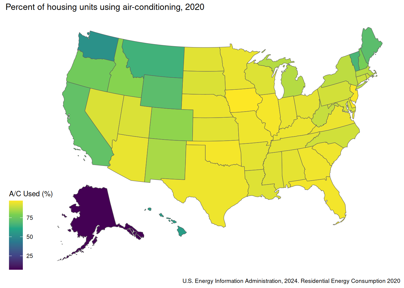
1 Yes Yes 0.794 0.777 0.810- Advanced bonus exercise What percentage of people used air-conditioning (A/C) in each state according to the RECS data? Extra bonus: Make a plot or map of this data by state - the usmap package may be useful.
Show code
ac_by_state <- recs_des %>%
  group_by(state_postal) %>%
  summarize(
    PctAC = survey_mean(ACUsed * 100)
  )

ac_by_state
# A tibble: 51 × 3
state_postal PctAC PctAC_se
<fct> <dbl> <dbl>
1 AL 93.5 1.52
2 AK 6.94 1.51
3 AZ 94.2 1.31
4 AR 93.4 1.86
5 CA 72.4 1.41
6 CO 81.7 2.15
7 CT 89.6 1.95
8 DE 97.0 1.51
9 DC 93.3 1.82
10 FL 95.8 0.785
# ℹ 41 more rowsShow code
library(usmap)

us_map() %>%
  left_join(ac_by_state, by = c("abbr" = "state_postal")) %>%
  ggplot(aes(fill = PctAC)) +
  geom_sf() +
  ggthemes::theme_map() +
  scale_fill_viridis_c(name = "A/C Used (%)") +
  labs(
    title = "Percent of housing units using air-conditioning, 2020",
    caption = "U.S. Energy Information Administration, 2024. Residential Energy Consumption 2020"
  )
Exercises - Part 2
- What is the design effect for the proportion of people who voted early?
Show code
anes_des %>%
  filter(!is.na(EarlyVote2020)) %>%
  group_by(EarlyVote2020) %>%
  summarize(
    p = survey_mean(deff = TRUE)
  ) %>%
  filter(EarlyVote2020 == "Yes")
# A tibble: 1 × 4
EarlyVote2020 p p_se p_deff
<fct> <dbl> <dbl> <dbl>
1 Yes 0.726 0.0247 1.50- What is the median temperature people set their thermostats to at night during the winter (using the RECS data)?
Show code
recs_des %>%
  summarize(
    med_night_winter_temp = survey_median(WinterTempNight, na.rm = TRUE)
  )
# A tibble: 1 × 2
med_night_winter_temp med_night_winter_temp_se
<dbl> <dbl>
1 68 0.250- People sometimes set their temperature differently over different seasons and during the day. What median temperatures do people set their thermostats to in the summer and winter, both during the day and at night? Include confidence intervals.
Show code
ests_med_temps <-
  recs_des %>%
  summarize(
    across(contains("Temp"), ~ survey_median(.x, na.rm = TRUE, vartype = "ci"))
  )

ests_med_temps
# A tibble: 1 × 18
WinterTempDay WinterTempDay_low WinterTempDay_upp WinterTempAway
<dbl> <dbl> <dbl> <dbl>
1 70 70 71 68
# ℹ 14 more variables: WinterTempAway_low <dbl>, WinterTempAway_upp <dbl>,
# WinterTempNight <dbl>, WinterTempNight_low <dbl>,
# WinterTempNight_upp <dbl>, SummerTempDay <dbl>, SummerTempDay_low <dbl>,
# SummerTempDay_upp <dbl>, SummerTempAway <dbl>, SummerTempAway_low <dbl>,
# SummerTempAway_upp <dbl>, SummerTempNight <dbl>, SummerTempNight_low <dbl>,
# SummerTempNight_upp <dbl>Show code
ests_med_temps %>%
  pivot_longer(cols = everything()) %>%
  separate_wider_delim(name, delim = "_", names = c("Var", "EstType"), too_few = "align_start") %>%
  mutate(
    EstType = if_else(is.na(EstType), "Median", EstType)
  ) %>%
  pivot_wider(names_from = EstType, values_from = value)
# A tibble: 6 × 4
Var Median low upp
<chr> <dbl> <dbl> <dbl>
1 WinterTempDay 70 70 71
2 WinterTempAway 68 68 69
3 WinterTempNight 68 68 69
4 SummerTempDay 72 72 73
5 SummerTempAway 74 74 75
6 SummerTempNight 72 72 73- What is the correlation between the temperature that people set their temperature at during the night and during the day in the summer?
Show code
recs_des %>%
  summarize(
    rho_temps = survey_corr(SummerTempNight, SummerTempDay, na.rm = TRUE)
  )
Warning: There was 1 warning in `dplyr::summarise()`.
ℹ In argument: `rho_temps = survey_corr(SummerTempNight, SummerTempDay, na.rm =
TRUE)`.
Caused by warning in `sweep()`:
! length(STATS) or dim(STATS) do not match dim(x)[MARGIN]# A tibble: 1 × 2
rho_temps rho_temps_se
<dbl> <dbl>
1 0.806 0.00806- What is the 1st, 2nd, and 3rd quartile of money spent on energy by Building America (BA) climate zone? Include the national estimates as well.
Show code
recs_des %>%
  group_by(ClimateRegion_BA) %>%
  cascade(
    EnergyCost = survey_quantile(TOTALDOL, quantiles = c(.25, .5, .75)),
    .fill = "National"
  )
# A tibble: 9 × 7
ClimateRegion_BA EnergyCost_q25 EnergyCost_q50 EnergyCost_q75
<fct> <dbl> <dbl> <dbl>
1 Mixed-Dry 1091. 1541. 2139.
2 Mixed-Humid 1317. 1840. 2462.
3 Hot-Humid 1094. 1622. 2233.
4 Hot-Dry 926. 1513. 2223.
5 Very-Cold 1195. 1986. 2955.
6 Cold 1213. 1756. 2422.
7 Marine 938. 1380. 1987.
8 Subarctic 2404. 3535. 5219.
9 National 1168. 1713. 2360.
# ℹ 3 more variables: EnergyCost_q25_se <dbl>, EnergyCost_q50_se <dbl>,
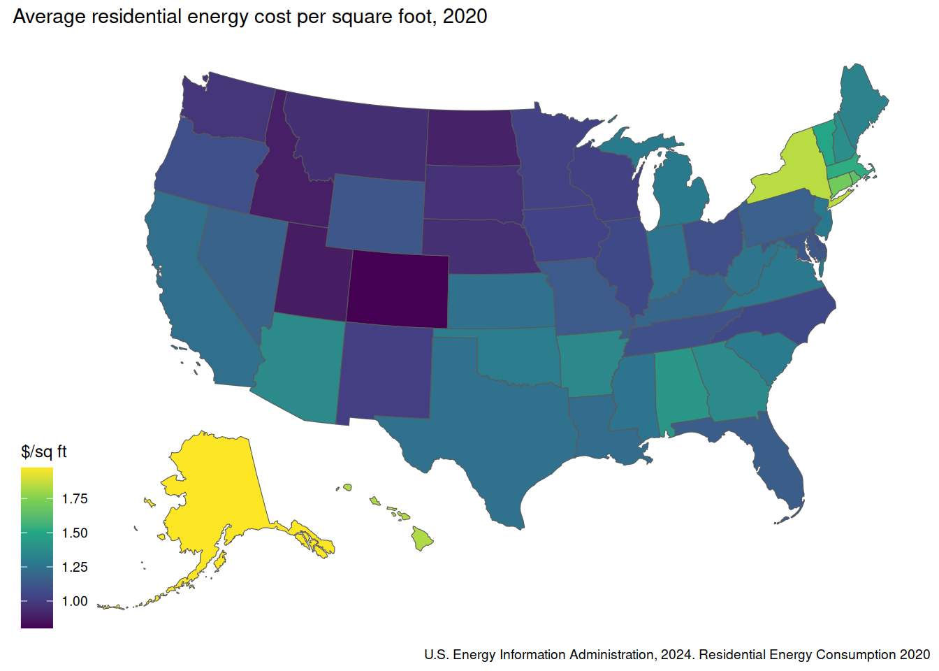
# EnergyCost_q75_se <dbl>- Advanced bonus exercise What is the average money spent on energy per square foot by state? Extra bonus: Make a plot or map of this data by state
Show code
energy_spend_by_state <- recs_des %>%
  group_by(state_postal) %>%
  summarize(
    EnergyCost = survey_mean(TOTALDOL / TOTSQFT_EN)
  )

energy_spend_by_state
# A tibble: 51 × 3
state_postal EnergyCost EnergyCost_se
<fct> <dbl> <dbl>
1 AL 1.42 0.0522
2 AK 1.98 0.0720
3 AZ 1.36 0.0326
4 AR 1.35 0.0529
5 CA 1.23 0.0202
6 CO 0.801 0.0274
7 CT 1.70 0.0606
8 DE 1.11 0.0481
9 DC 1.14 0.0332
10 FL 1.15 0.0246
# ℹ 41 more rowsShow code
library(usmap)

us_map() %>%
  left_join(energy_spend_by_state, by = c("abbr" = "state_postal")) %>%
  ggplot(aes(fill = EnergyCost)) +
  geom_sf() +
  ggthemes::theme_map() +
  scale_fill_viridis_c(name = "$/sq ft") +
  labs(
    title = "Average residential energy cost per square foot, 2020",
    caption = "U.S. Energy Information Administration, 2024. Residential Energy Consumption 2020"
  )