Tidy Data,
Weighted Insights

Analyzing Complex Survey Data in R

About us

Stephanie Zimmer

RTI International

Rebecca Powell

Fors Marsh

Isabella Velásquez

Posit

Overview

• Using R for survey analysis
• Setting up your analysis
• Introducing databases
• Calculating means
• Conducting t-tests
• Creating tables
• Wrap up

Introduction to {survey} and {srvyr}

R packages for survey analysis

• {survey} package first on CRAN in 2003
  • descriptive analysis
  • statistical testing
  • modeling
  • weighting
• {srvyr} package first on CRAN in 2016
  • “wrapper” for {survey} with {tidyverse}-style syntax
  • only descriptive analysis
• {gtsummary} package first on CRAN in 2016
  • creates publication-ready tables from survey data
  • currently cannot handle replicate weights

• R packages are a collection of functions
• This is not an exhaustive list of packages that work with survey data
• Several packages for imputation, more complex weighting, and more
• gtsummary won’t be discussed today

Comparison with dplyr

• dplyr: summary functions called within summarize()

dplyr

towny %>%
  group_by(status) %>%
  summarize(
    area_mean = mean(land_area_km2),
    area_median = median(land_area_km2)
  )

# A tibble: 2 × 3
  status      area_mean area_median
  <chr>           <dbl>       <dbl>
1 lower-tier       362.        310.
2 single-tier      388.        194.

Comparison with dplyr

• srvyr: survey_*() functions called with summarize()

srvyr

apistrat_des %>%
  group_by(stype) %>%
  summarize(
    api00_mean = survey_mean(api00),
    api00_med = survey_median(api00)
  )

# A tibble: 3 × 5
  stype api00_mean api00_mean_se api00_med api00_med_se
  <fct>      <dbl>         <dbl>     <dbl>        <dbl>
1 E           674.          12.5       671         20.7
2 H           626.          15.5       635         21.6
3 M           637.          16.6       648         24.1

• If you already use {tidyverse}/{dplyr}, the syntax {srvyr} will come easily
• Functions commonly used like group_by, filter, and summarize also used in srvyr
• Note that the survey estimates also generate standard deviations - can also add options to get CIs, deffs, and variances

Survey analysis process

Steps for descriptive analysis

1. Create a tbl_svy object (a survey object) using: as_survey_design() or as_survey_rep()

2. Subset data (if needed) using filter() (to create subpopulations)

3. Specify domains of analysis using group_by()

4. Within summarize(), specify variables to calculate, including means, totals, proportions, quantiles, and more

• Survey object involves specifying weights, strata and/or clusters (PSUs) OR replicate weights
• Survey object can be used over and over for the same data and different analyses
• This is necessary for getting appropriate weighted estimates and standard errors. More public use files are providing this syntax
• Can also use cascade() instead of summarize() to get the total row

Steps for testing

1. Create a tbl_svy object (a survey object) using: as_survey_design() or as_survey_rep()

2. Subset data (if needed) using filter() (to create subpopulations)

3. Use svyttest() for comparisons of proportions and means, svygofchisq() for GOF test, or svychisq() for test of independence and test of homogeneity

• Only last step changes from descriptive analysis.

Steps for modeling

1. Create a tbl_svy object (a survey object) using: as_survey_design() or as_survey_rep()

2. Subset data (if needed) using filter() (to create subpopulations)

3. Use svyglm() for linear models and logistic models, svycoxph() for Cox proportional-hazards, svykm() for Kaplan-Meier, svyloglin() for log-linear models, svyolr() for multinomial

• Only last step changes from descriptive analysis. Syntax mirrors glm, coxph, etc functions for non-survey data

Load packages and data

Load packages

# install.packages(c("survey", "srvyr", "duckdb", "dbplyr", "gt"))
library(survey)
library(srvyr)
library(duckdb)
library(dbplyr)
library(gt)

Today’s data

Data from the 2021 Census of Population conducted by Statistics Canada

• Public-use microdata from the long-form census sample, named data_donnees_2021_ind_v2.csv
• Analysis uses survey weights and replicate weights provided with the data
• 980,868 rows and 144 columns (604 MB)
• Available online at: https://www150.statcan.gc.ca/n1/pub/98m0001x/index-eng.htm

Database detour

• Initiate DuckDB database
• Load CSV into database - data does NOT go into RAM
• nread creates a small check that the number of records loaded as expected

con <- dbConnect(duckdb())
nread <- duckdb_read_csv(
  conn = con,
  name = "c2021_ind",
  here::here("RawDat", "data_donnees_2021_ind_v2.csv")
)

nread

[1] 980868

• For this example, we create a duckdb database. You could be pointing to existing database

Database tables in R

• Make a R object pointing to the table
• This R object is NOT a data.frame

c2021_ind_db <- dplyr::tbl(con, I("c2021_ind"))
object.size(c2021_ind_db) %>% print(units="Gb")

0 Gb

c2021_ind_db

# A query:  ?? x 144
# Database: DuckDB 1.4.4 [root@Darwin 22.5.0:R 4.5.2/:memory:]
   PPSORT ABOID AGEGRP AGEIMM ATTSCH BFNMEMB BedRm CFInc CFInc_AT CFSTAT   CHDBN
    <int> <int>  <int>  <int>  <int>   <int> <int> <int>    <int>  <int>   <int>
 1      1     6     13      7      1       0     4    30       27      2 8.89 e7
 2      2     6     11      5      1       0     3    18       18      2 1.15 e4
 3      3     1     13     99      1       0     0     7        7      6 1.000e8
 4      4     6     16     99      1       0     4    15       15      2 1.000e8
 5      5     6     18     99      1       0     3    13       13      3 1.000e8
 6      6     2     16     99      1       0     4     1        1      7 1.000e8
 7      7     6     16     99      1       0     3    10       10      1 1.000e8
 8      8     6     16      7      1       0     4    30       27      1 1.000e8
 9      9     6     11     99      1       0     4    25       24      2 1.000e8
10     10     6     12      6      1       0     4    22       22      2 1.000e8
# ℹ more rows
# ℹ 133 more variables: CIP2021 <int>, CIP2021_STEM_SUM <int>, CMA <int>,
#   CONDO <int>, COVID_ERB <int>, COW <int>, CQPPB <int>, CapGn <int>,
#   CfSize <int>, ChldC <int>, CitOth <int>, Citizen <int>, DIST <int>,
#   DPGRSUM <int>, DTYPE <int>, EFDecile <int>, EFInc <int>, EFInc_AT <int>,
#   EICBN <int>, ETHDER <int>, EfDIMBM_2018 <int>, EfSize <int>, EmpIn <int>,
#   FOL <int>, FPTWK <int>, Gender <int>, GENSTAT <int>, GovtI <int>, …

Design object

• After loading packages and data
• First step is to create design object
• Account for the sampling design or replicate weights
• Accurately calculate the estimates (using the correct underlying formulas)
• There are two functions for creating the design object depending on if using replicate weights or not

Syntax: replicate weights

For studies with replicate weights, create the survey object using the as_survey_rep() function.

as_survey_rep(
  .data,
  variables = NULL,
  weights = NULL,
  repweights = NULL,
  type = c("BRR", "Fay", "JK1", "JKn", "bootstrap", 
           "successive-difference", "ACS", "other"),
  combined_weights = TRUE,
  rho = NULL,
  bootstrap_average = NULL,
  scale = NULL,
  rscales = NULL,
  fpc = NULL,
  fpctype = c("fraction", "correction"),
  mse = getOption("survey.replicates.mse"),
  degf = NULL,
  ...
)

Syntax: replicate weights

For studies with replicate weights, create the survey object using the as_survey_rep() function.

as_survey_rep(
  .data,
  variables = NULL,
  weights = NULL,
  repweights = NULL,
  type = c("BRR", "Fay", "JK1", "JKn", "bootstrap", 
           "successive-difference", "ACS","other"),
  combined_weights = TRUE,
  rho = NULL,
  bootstrap_average = NULL,
  scale = NULL,
  rscales = NULL,
  fpc = NULL,
  fpctype = c("fraction", "correction"),
  mse = getOption("survey.replicates.mse"),
  degf = NULL,
  ...
)

• As with the first function, there is a weights argument for the main analytic weight
• Also has the repweights argument to indicate the variables that hold the replicate weights
• Need to include the type of replicate weights: Balanced Repeated Replicates (BRR), Fay, Jackknife (JK), etc.
• Have separate arguments for the various parameters for the replicate weights: rho, scale, etc.

Implementation - design object

cens_des <- c2021_ind_db %>%
  as_survey_rep(
1    weights = WEIGHT,
2    repweights = WT1:WT16,
    type = "other",
3    scale = 1/35,
4    mse = TRUE,
5    rscales = 1)

1

Main analytic weight in WEIGHT variable

2

Replicate weights start with WT1-WT16 variables

3

Scaling per documentation is dividing by 35

4

Center replicates around main estimate, not mean of replicates

5

When specifying type="other", must specify rscales

• Using the documention for the 2021 Canadian Census, learn the variable names for the weights, the type, and the scale

Results

• Design object contains all the design data (i.e., replicate weights)
• Remaining data is in the database only
• Efficiency opportunity: specify degrees of freedom when creating design object

object.size(cens_des) %>% print(units="Gb")

0.2 Gb

cens_des

Call: Called via srvyr
with 16 replicates and MSE variances.
Sampling variables:
  - repweights: `WT1 + WT2 + WT3 + WT4 + WT5 + WT6 + WT7 + WT8 + WT9 + WT10 +
    WT11 + WT12 + WT13 + WT14 + WT15 + WT16` 
  - weights: WEIGHT 
Data variables: 
  - PPSORT (int), ABOID (int), AGEGRP (int), AGEIMM (int), ATTSCH (int),
    BFNMEMB (int), BedRm (int), CFInc (int), CFInc_AT (int), CFSTAT (int),
    CHDBN (int), CIP2021 (int), CIP2021_STEM_SUM (int), CMA (int), CONDO (int),
    COVID_ERB (int), COW (int), CQPPB (int), CapGn (int), CfSize (int), ChldC
    (int), CitOth (int), Citizen (int), DIST (int), DPGRSUM (int), DTYPE (int),
    EFDecile (int), EFInc (int), EFInc_AT (int), EICBN (int), ETHDER (int),
    EfDIMBM_2018 (int), EfSize (int), EmpIn (int), FOL (int), FPTWK (int),
    Gender (int), GENSTAT (int), GovtI (int), GTRfs (int), HCORENEED_IND (int),
    HDGREE (int), HHInc (int), HHInc_AT (int), HHMRKINC (int), HHSIZE (int),
    HHTYPE (int), HLMOSTEN (int), HLMOSTFR (int), HLMOSTNO (int), HLREGEN
    (int), HLREGFR (int), HLREGNO (int), IMMCAT5 (int), IMMSTAT (int), IncTax
    (int), Invst (int), JOBPERM (int), KOL (int), LFACT (int), LICO_BT (int),
    LICO_AT (int), LIPROGTYPE (int), LI_ELIG_OML_U18 (int), LOCSTUD (int),
    LOC_ST_RES (int), LSTWRK (int), LWMOSTEN (int), LWMOSTFR (int), LWMOSTNO
    (int), LWREGEN (int), LWREGFR (int), LWREGNO (int), LoLIMA (int), LoLIMB
    (int), LoMBM_2018 (int), MODE (int), MTNEN (int), MTNFR (int), MTNNO (int),
    MarStH (int), Mob1 (int), Mob5 (int), MrkInc (int), NAICS (int), NOC21
    (int), NOL (int), NOS (int), OASGI (int), OtInc (int), PKID25 (int),
    PKID0_1 (int), PKID15_24 (int), PKID2_5 (int), PKID6_14 (int), PKIDS (int),
    POB (int), POBPAR1 (int), POBPAR2 (int), POWST (int), PR (int), PR1 (int),
    PR5 (int), PresMortG (int), PRIHM (int), PWDUR (int), PWLEAVE (int), PWOCC
    (int), PWPR (int), REGIND (int), Relig (int), REPAIR (int), ROOM (int),
    Retir (int), SHELCO (int), SSGRAD (int), Subsidy (int), SempI (int), Tenur
    (int), TotInc (int), TotInc_AT (int), VISMIN (int), Value (int), WKSWRK
    (int), WRKACT (int), Wages (int), YRIM (int), WEIGHT (dbl), WT1 (dbl), WT2
    (dbl), WT3 (dbl), WT4 (dbl), WT5 (dbl), WT6 (dbl), WT7 (dbl), WT8 (dbl),
    WT9 (dbl), WT10 (dbl), WT11 (dbl), WT12 (dbl), WT13 (dbl), WT14 (dbl), WT15
    (dbl), WT16 (dbl)

Calculate means

Syntax

The survey_mean() calculates means while taking into account the survey design elements.

survey_mean(
  x,
  na.rm = FALSE,
  vartype = c("se", "ci", "var", "cv"),
  level = 0.95,
  proportion = FALSE,
  prop_method = c("logit", "likelihood", "asin", "beta", "mean"),
  deff = FALSE,
  df = NULL
)

Implementation

Calculate the estimated average cost of housing (SHELCO) in Canada:

cens_des %>%
  summarize(housing_cost = survey_mean(SHELCO, 
                                       vartype = c("se", "ci"))) 

• Use the survey design object, not raw data

Implementation

Calculate the estimated average cost of housing (SHELCO) in Canada:

cens_des %>%
  summarize(housing_cost = survey_mean(SHELCO, 
                                       vartype = c("se", "ci"))) 

• Use the survey design object, not raw data
• Call survey_mean() within summarize() function

Implementation

Calculate the estimated average cost of housing (SHELCO) in Canada:

cens_des %>%
  summarize(housing_cost = survey_mean(SHELCO, 
                                       vartype = c("se", "ci"))) 

• Use the survey design object, not raw data
• Call survey_mean() within summarize() function
• Specify the type of variance output, here we output the standard error and confidence interval

Results

Calculate the estimated average cost of housing (SHELCO) in Canada:

cens_des %>%
  summarize(housing_cost = survey_mean(SHELCO, 
                                       vartype = c("se", "ci"))) 

# A tibble: 1 × 4
  housing_cost housing_cost_se housing_cost_low housing_cost_upp
         <dbl>           <dbl>            <dbl>            <dbl>
1        1592.            1.12            1590.            1594.

• Estimated average cost of housing cost is in the first column
• Standard error is in the second column
• Confidence interval is in the third and fourth columns (lower bound, upper bound)
• This is the standard R output, we will show later on how to make these into prettier tables

Calculate means with groups

Calculate the estimated average cost of housing (SHELCO) in Canada by each province (PR) by including a group_by() function with the variable of interest before the summarize() function:

cens_des %>%
  group_by(PR) %>%
  summarize(housing_cost = survey_mean(SHELCO, 
                                       vartype = c("se", "ci"))) 

# A tibble: 11 × 5
      PR housing_cost housing_cost_se housing_cost_low housing_cost_upp
   <int>        <dbl>           <dbl>            <dbl>            <dbl>
 1    10        1113.            7.75            1097.            1130.
 2    11        1126.            8.33            1108.            1143.
 3    12        1187.            5.14            1177.            1198.
 4    13        1011.            3.42            1004.            1019.
 5    24        1211.            1.77            1207.            1215.
 6    35        1810.            2.05            1806.            1814.
 7    46        1274.            6.39            1260.            1287.
 8    47        1350.            4.80            1340.            1360.
 9    48        1760.            2.70            1755.            1766.
10    59        1845.            3.75            1837.            1853.
11    70        1432.           18.0             1394.            1471.

• When working with subgroups, need to subset (filter()) or define groups (group_by()) before calculating the estimates
• Here we are interested in cost of housing for each province
• Output has a row for each province
• Missing labels

Database detour: Factors/Labelled Data

• Working with databases is fast and helpful with large data! BUT…

• Cannot have labelled data or factors, so our output may not be meaningful

• Couple of options:

  1. Create a new variable that is the labelled data
  2. After completing your analyses, label the final tables

Factors/Labelled Data - Option 1

cens_des %>%
  mutate(Province = case_when(PR == 10 ~ "Newfoundland and Labrador",
                              PR == 11 ~ "Prince Edward Island",
                              PR == 12 ~ "Nova Scotia",
                              PR == 13 ~ "New Brunswick",
                              PR == 24 ~ "Quebec",
                              PR == 35 ~ "Ontario",
                              PR == 46 ~ "Manitoba",
                              PR == 47 ~ "Saskatchewan",
                              PR == 48 ~ "Alberta",
                              PR == 59 ~ "British Columbia",
                              PR == 70 ~ "Northern Canada")) %>% 
  group_by(Province) %>%
  summarize(housing_cost = survey_mean(SHELCO, 
                                       vartype = c("se", "ci"))) 

# A tibble: 11 × 5
   Province       housing_cost housing_cost_se housing_cost_low housing_cost_upp
   <chr>                 <dbl>           <dbl>            <dbl>            <dbl>
 1 Alberta               1760.            2.70            1755.            1766.
 2 British Colum…        1845.            3.75            1837.            1853.
 3 Manitoba              1274.            6.39            1260.            1287.
 4 New Brunswick         1011.            3.42            1004.            1019.
 5 Newfoundland …        1113.            7.75            1097.            1130.
 6 Northern Cana…        1432.           18.0             1394.            1471.
 7 Nova Scotia           1187.            5.14            1177.            1198.
 8 Ontario               1810.            2.05            1806.            1814.
 9 Prince Edward…        1126.            8.33            1108.            1143.
10 Quebec                1211.            1.77            1207.            1215.
11 Saskatchewan          1350.            4.80            1340.            1360.

• Output auto sorts alphabetically

Factors/Labelled Data - Option 2

cens_des %>%
  group_by(PR) %>%
  summarize(housing_cost = survey_mean(SHELCO, 
                                       vartype = c("se", "ci"))) %>%
  mutate(PR = factor(as.character(PR),
                     levels=c("10", "11", "12", "13", "24", "35", "46",
                              "47", "48", "59", "70"),
                     labels=c("Newfoundland and Labrador", "Prince Edward Island", 
                              "Nova Scotia", "New Brunswick", "Quebec", "Ontario",
                              "Manitoba", "Saskatchewan", "Alberta", 
                              "British Columbia", "Northern Canada")))

# A tibble: 11 × 5
   PR             housing_cost housing_cost_se housing_cost_low housing_cost_upp
   <fct>                 <dbl>           <dbl>            <dbl>            <dbl>
 1 Newfoundland …        1113.            7.75            1097.            1130.
 2 Prince Edward…        1126.            8.33            1108.            1143.
 3 Nova Scotia           1187.            5.14            1177.            1198.
 4 New Brunswick         1011.            3.42            1004.            1019.
 5 Quebec                1211.            1.77            1207.            1215.
 6 Ontario               1810.            2.05            1806.            1814.
 7 Manitoba              1274.            6.39            1260.            1287.
 8 Saskatchewan          1350.            4.80            1340.            1360.
 9 Alberta               1760.            2.70            1755.            1766.
10 British Colum…        1845.            3.75            1837.            1853.
11 Northern Cana…        1432.           18.0             1394.            1471.

• Output maintains ordering
• Needs to be after the summarize, or it will try to edit the database and will not work.

Conduct t-tests

Syntax

Use the svyttest() function to compare two proportions or means.

Syntax:

svyttest(
  formula,
  design,
  ...
)

• Similar to t.test() function in base R with the formula and the data arguments
• Design object is the second argument

Dot notation

• Design object is not the first argument
• Need to specify with dot notation in pipes

design_obj %>%
  svyttest(formula = var1 ~ var2,
           design = .)

design_obj %>%
  svyttest(design = .,
           formula = var1 ~ var2)

Syntax pipeline with databases

1. Select the variables involved in the test
2. Collect the design object
3. Perform the test

design_obj %>%
  select(var1, var2) %>%
  collect() %>%
  svyttest(formula = var1 ~ var2,
           design = .)

Implementation: one-sample t-test

Is the proportion of females¹ in Canada different from 50% among those 65 years old and over?

cens_des %>%
  filter(between(AGEGRP, 17, 21)) %>%
  mutate(Woman=if_else(Gender==1, 1, 0)) %>%
  summarize(
    WomenPct=survey_mean(Woman, proportion = TRUE, vartype = "ci")
  )

# A tibble: 1 × 3
  WomenPct WomenPct_low WomenPct_upp
     <dbl>        <dbl>        <dbl>
1    0.532        0.529        0.535

• start by looking at the average age using survey_mean()
• filtering to 5 levels of AGEGRP (17-21)
• create new binary variable called ‘Woman’

1. measured on the binary

Implementation: one-sample t-test

Is the proportion of women in Canada different from 50% among those 65 years old and over?

cens_des %>%
  filter(between(AGEGRP, 17, 21)) %>%
  mutate(Woman=if_else(Gender==1, 1, 0)) %>% 
  select(Woman) %>%
  collect() %>%
  svyttest(
    formula = Woman - 0.5 ~ 0,
    design = .) %>%
  broom::tidy()

• Subset data to those age 65 and older
• Specify Woman variable as 0/1 to calculate proportion

Implementation: one-sample t-test

Is the proportion of women in Canada different from 50% among those 65 years old and over?

cens_des %>%
  filter(between(AGEGRP, 17, 21)) %>%
  mutate(Woman=if_else(Gender==1, 1, 0)) %>% 
  select(Woman) %>%
  collect() %>%
  svyttest(
    formula = Woman - 0.5 ~ 0,
    design = .) %>%
  broom::tidy()

• Subset data to those age 65 and older
• Specify Woman variable as 0/1 to calculate proportion
• Select the variable needed for test

Implementation: one-sample t-test

Is the proportion of women in Canada different from 50% among those 65 years old and over?

cens_des %>%
  filter(between(AGEGRP, 17, 21)) %>%
  mutate(Woman=if_else(Gender==1, 1, 0)) %>% 
  select(Woman) %>%
  collect() %>%
  svyttest(
    formula = Woman - 0.5 ~ 0,
    design = .) %>%
  broom::tidy()

• Subset data to those age 65 and older
• Specify Woman variable as 0/1 to calculate proportion
• Select the variable needed for test
• Bring data out of database to R for testing

Implementation: one-sample t-test

Is the proportion of women in Canada different from 50% among those 65 years old and over?

cens_des %>%
  filter(between(AGEGRP, 17, 21)) %>%
  mutate(Woman=if_else(Gender==1, 1, 0)) %>% 
  select(Woman) %>%
  collect() %>%
  svyttest(
    formula = Woman - 0.5 ~ 0,
    design = .) %>%
  broom::tidy()

• Subset data to those age 65 and older
• Specify Woman variable as 0/1 to calculate proportion
• Select the variable needed for test
• Bring data out of database to R for testing
• Specify one-sided formula, always compared to 0

Implementation: one-sample t-test

Is the proportion of women in Canada different from 50% among those 65 years old and over?

cens_des %>%
  filter(between(AGEGRP, 17, 21)) %>%
  mutate(Woman=if_else(Gender==1, 1, 0)) %>% 
  select(Woman) %>%
  collect() %>%
  svyttest(
    formula = Woman - 0.5 ~ 0,
    design = .) %>%
  broom::tidy()

• Subset data to those age 65 and older
• Specify Woman variable as 0/1 to calculate proportion
• Select the variable needed for test
• Bring data out of database to R for testing
• Specify one-sided formula, always compared to 0
• broom::tidy() returns the test as a nice tibble

Implementation: one-sample t-test

Is the proportion of women in Canada different from 50% among those 65 years old and over?

cens_des %>%
  filter(between(AGEGRP, 17, 21)) %>%
  mutate(Woman=if_else(Gender==1, 1, 0)) %>%
  select(Woman) %>%
  collect() %>%
  svyttest(
    formula = Woman - 0.5 ~ 0,
    design = .) %>%
  broom::tidy()

# A tibble: 1 × 8
  estimate statistic  p.value parameter conf.low conf.high method    alternative
     <dbl>     <dbl>    <dbl>     <dbl>    <dbl>     <dbl> <chr>     <chr>      
1   0.0323      23.8 1.03e-12        14   0.0294    0.0353 Design-b… two.sided  

Implementation: two-sample t-test

On average, is there a significant difference in salary between adult women and men among those who were employees?

First, look at the estimated average employment income for women and men, who are adult full-time employees.

cenc_des_ftw_adult <- cens_des %>%
  filter(between(AGEGRP, 7, 21), 
         COW == 1, 
         !EmpIn %in% c(88888888, 99999999), 
         FPTWK == 1) %>%
  mutate(GenderC=if_else(Gender==1, "Woman", "Man"))

cenc_des_ftw_adult %>%
  group_by(GenderC) %>%
  summarize(
    EmpInMn = survey_mean(EmpIn)
  )

# A tibble: 2 × 3
  GenderC EmpInMn EmpInMn_se
  <chr>     <dbl>      <dbl>
1 Man      74129.       196.
2 Woman    57148.       147.

• AGEGRP (Age groups) 7-21 gives us adults
• COW (Class of Worker) 1 gives us “Employees” - not selfemployeed, unpaid
• EmpIn removing missing data
• FPTWK (full time/part time designation) 1 gives us mostly full time in 2020

Implementation: two-sample t-test

Test if the employment income is significantly different for women and men:

cenc_des_ftw_adult %>%
  select(EmpIn, GenderC)  %>%
  collect() %>%
  svyttest(
    formula = EmpIn ~ GenderC,
    design = .
  ) %>%
    broom::tidy()

# A tibble: 1 × 8
  estimate statistic  p.value parameter conf.low conf.high method    alternative
     <dbl>     <dbl>    <dbl>     <dbl>    <dbl>     <dbl> <chr>     <chr>      
1  -16982.     -60.1 2.66e-18        14  -17587.   -16376. Design-b… two.sided  

• forumla becomes y ~ x: income ~ group

Create tables

Syntax

With the {gt} package, supply the input data table to gt() and add options to modify and format your table.

data %>%
  gt() %>%
  ... add options here...

Implementation

Create a table for estimated monthly cost of housing in Canada by province:

cens_tab <- cens_des %>%
  group_by(PR) %>%
  summarize(housing_cost =
              survey_mean(SHELCO, vartype = c("se", "ci"))) %>%
  mutate(PR = as.character(PR))

cens_tab

# A tibble: 11 × 5
   PR    housing_cost housing_cost_se housing_cost_low housing_cost_upp
   <chr>        <dbl>           <dbl>            <dbl>            <dbl>
 1 10           1113.            7.75            1097.            1130.
 2 11           1126.            8.33            1108.            1143.
 3 12           1187.            5.14            1177.            1198.
 4 13           1011.            3.42            1004.            1019.
 5 24           1211.            1.77            1207.            1215.
 6 35           1810.            2.05            1806.            1814.
 7 46           1274.            6.39            1260.            1287.
 8 47           1350.            4.80            1340.            1360.
 9 48           1760.            2.70            1755.            1766.
10 59           1845.            3.75            1837.            1853.
11 70           1432.           18.0             1394.            1471.

Implementation

Pipe (%>%) your data frame (cens_tab) into the gt() function:

cens_tab %>%
  gt()

PR	housing_cost	housing_cost_se	housing_cost_low	housing_cost_upp
10	1113.273	7.748895	1096.757	1129.790
11	1125.558	8.331108	1107.800	1143.315
12	1187.458	5.138334	1176.506	1198.410
13	1011.460	3.418450	1004.174	1018.746
24	1211.113	1.771247	1207.337	1214.888
35	1809.889	2.046193	1805.527	1814.250
46	1273.580	6.386941	1259.967	1287.193
47	1350.052	4.799534	1339.822	1360.282
48	1760.305	2.696103	1754.559	1766.052
59	1844.768	3.753446	1836.768	1852.768
70	1432.166	18.025602	1393.745	1470.586

Implementation

Continue adding to your table, for example, designating Province as a “stub”:

cens_tab %>%
  gt(rowname_col = "PR")

	housing_cost	housing_cost_se	housing_cost_low	housing_cost_upp
10	1113.273	7.748895	1096.757	1129.790
11	1125.558	8.331108	1107.800	1143.315
12	1187.458	5.138334	1176.506	1198.410
13	1011.460	3.418450	1004.174	1018.746
24	1211.113	1.771247	1207.337	1214.888
35	1809.889	2.046193	1805.527	1814.250
46	1273.580	6.386941	1259.967	1287.193
47	1350.052	4.799534	1339.822	1360.282
48	1760.305	2.696103	1754.559	1766.052
59	1844.768	3.753446	1836.768	1852.768
70	1432.166	18.025602	1393.745	1470.586

Implementation

Add a title:

cens_tab %>%
  gt(rowname_col = "PR") %>%
  tab_header(title = "Monthly cost of housing in Canada by province")

Monthly cost of housing in Canada by province
	housing_cost	housing_cost_se	housing_cost_low	housing_cost_upp
10	1113.273	7.748895	1096.757	1129.790
11	1125.558	8.331108	1107.800	1143.315
12	1187.458	5.138334	1176.506	1198.410
13	1011.460	3.418450	1004.174	1018.746
24	1211.113	1.771247	1207.337	1214.888
35	1809.889	2.046193	1805.527	1814.250
46	1273.580	6.386941	1259.967	1287.193
47	1350.052	4.799534	1339.822	1360.282
48	1760.305	2.696103	1754.559	1766.052
59	1844.768	3.753446	1836.768	1852.768
70	1432.166	18.025602	1393.745	1470.586

Implementation

Add more informative labels:

cens_tab %>%
  gt(rowname_col = "PR") %>%
  tab_header(title = "Cost of housing in Canada by province") %>%
  cols_label(
    housing_cost = "Average",
    housing_cost_se = "SE",
    housing_cost_low = "Lower",
    housing_cost_upp = "Upper"
  )

Implementation

Cost of housing in Canada by province
	Average	SE	Lower	Upper
10	1113.273	7.748895	1096.757	1129.790
11	1125.558	8.331108	1107.800	1143.315
12	1187.458	5.138334	1176.506	1198.410
13	1011.460	3.418450	1004.174	1018.746
24	1211.113	1.771247	1207.337	1214.888
35	1809.889	2.046193	1805.527	1814.250
46	1273.580	6.386941	1259.967	1287.193
47	1350.052	4.799534	1339.822	1360.282
48	1760.305	2.696103	1754.559	1766.052
59	1844.768	3.753446	1836.768	1852.768
70	1432.166	18.025602	1393.745	1470.586

Implementation

Label certain columns using spanners:

cens_tab %>%
  gt(rowname_col = "PR") %>%
  tab_header(title = "Cost of housing in Canada by province") %>%
  cols_label(
    housing_cost = "Average",
    housing_cost_se = "SE",
    housing_cost_low = "Lower",
    housing_cost_upp = "Upper"
  ) %>%
  tab_spanner(
    label = "Dollars",
    columns = c(housing_cost, housing_cost_se, housing_cost_low, housing_cost_upp)
  )

Implementation

Cost of housing in Canada by province
	Dollars
	Average	SE	Lower	Upper
10	1113.273	7.748895	1096.757	1129.790
11	1125.558	8.331108	1107.800	1143.315
12	1187.458	5.138334	1176.506	1198.410
13	1011.460	3.418450	1004.174	1018.746
24	1211.113	1.771247	1207.337	1214.888
35	1809.889	2.046193	1805.527	1814.250
46	1273.580	6.386941	1259.967	1287.193
47	1350.052	4.799534	1339.822	1360.282
48	1760.305	2.696103	1754.559	1766.052
59	1844.768	3.753446	1836.768	1852.768
70	1432.166	18.025602	1393.745	1470.586

Implementation

Format numbers with the fmt_*() functions:

cens_tab %>%
  gt(rowname_col = "PR") %>%
  tab_header(title = "Cost of housing in Canada by province") %>%
  cols_label(
    housing_cost = "Average",
    housing_cost_se = "SE",
    housing_cost_low = "Lower",
    housing_cost_upp = "Upper"
  ) %>%
  tab_spanner(
    label = "Dollars",
    columns = c(housing_cost, housing_cost_se, housing_cost_low, housing_cost_upp)
  ) %>%
  fmt_number(decimals = 2)

Implementation

Cost of housing in Canada by province
	Dollars
	Average	SE	Lower	Upper
10	1,113.27	7.75	1,096.76	1,129.79
11	1,125.56	8.33	1,107.80	1,143.31
12	1,187.46	5.14	1,176.51	1,198.41
13	1,011.46	3.42	1,004.17	1,018.75
24	1,211.11	1.77	1,207.34	1,214.89
35	1,809.89	2.05	1,805.53	1,814.25
46	1,273.58	6.39	1,259.97	1,287.19
47	1,350.05	4.80	1,339.82	1,360.28
48	1,760.31	2.70	1,754.56	1,766.05
59	1,844.77	3.75	1,836.77	1,852.77
70	1,432.17	18.03	1,393.75	1,470.59

Implementation

Change row labels (without editing your data):

cens_tab %>%
  gt(rowname_col = "PR") %>%
  tab_header(title = "Cost of housing in Canada by province") %>%
  cols_label(
    housing_cost = "Average",
    housing_cost_se = "SE",
    housing_cost_low = "Lower",
    housing_cost_upp = "Upper"
  ) %>%
  tab_spanner(
    label = "Dollars",
    columns = c(housing_cost, housing_cost_se, housing_cost_low, housing_cost_upp)
  ) %>%
  fmt_number(decimals = 2) %>%
  text_case_match(
    "10" ~ "Newfoundland and Labrador",
    "11" ~ "Prince Edward Island",
    "12" ~ "Nova Scotia",
    "13" ~ "New Brunswick",
    "24" ~ "Quebec", 
    "35" ~ "Ontario",
    "46" ~ "Manitoba",
    "47" ~ "Saskatchewan",
    "48" ~ "Alberta",
    "59" ~ "British Columbia",
    "70" ~ "Northern Canada",
    .locations = cells_stub()
  )

Implementation

Cost of housing in Canada by province
	Dollars
	Average	SE	Lower	Upper
Newfoundland and Labrador	1,113.27	7.75	1,096.76	1,129.79
Prince Edward Island	1,125.56	8.33	1,107.80	1,143.31
Nova Scotia	1,187.46	5.14	1,176.51	1,198.41
New Brunswick	1,011.46	3.42	1,004.17	1,018.75
Quebec	1,211.11	1.77	1,207.34	1,214.89
Ontario	1,809.89	2.05	1,805.53	1,814.25
Manitoba	1,273.58	6.39	1,259.97	1,287.19
Saskatchewan	1,350.05	4.80	1,339.82	1,360.28
Alberta	1,760.31	2.70	1,754.56	1,766.05
British Columbia	1,844.77	3.75	1,836.77	1,852.77
Northern Canada	1,432.17	18.03	1,393.75	1,470.59

Implementation

Finish by adding a source ✨

cens_tab %>%
  gt(rowname_col = "PR") %>%
  tab_header(title = "Cost of housing in Canada by province") %>%
  cols_label(
    housing_cost = "Average",
    housing_cost_se = "SE",
    housing_cost_low = "Lower",
    housing_cost_upp = "Upper"
  ) %>%
  tab_spanner(
    label = "Dollars",
    columns = c(housing_cost, housing_cost_se, housing_cost_low, housing_cost_upp)
  ) %>%
  fmt_number(decimals = 2) %>%
  text_case_match(
    "10" ~ "Newfoundland and Labrador",
    "11" ~ "Prince Edward Island",
    "12" ~ "Nova Scotia",
    "13" ~ "New Brunswick",
    "24" ~ "Quebec", 
    "35" ~ "Ontario",
    "46" ~ "Manitoba",
    "47" ~ "Saskatchewan",
    "48" ~ "Alberta",
    "59" ~ "British Columbia",
    "70" ~ "Northern Canada",
    .locations = cells_stub()
  ) %>%
  tab_source_note(source_note = "Statistica Canada. 2021 Canadian Census of Population.")

Implementation

Cost of housing in Canada by province
	Dollars
	Average	SE	Lower	Upper
Newfoundland and Labrador	1,113.27	7.75	1,096.76	1,129.79
Prince Edward Island	1,125.56	8.33	1,107.80	1,143.31
Nova Scotia	1,187.46	5.14	1,176.51	1,198.41
New Brunswick	1,011.46	3.42	1,004.17	1,018.75
Quebec	1,211.11	1.77	1,207.34	1,214.89
Ontario	1,809.89	2.05	1,805.53	1,814.25
Manitoba	1,273.58	6.39	1,259.97	1,287.19
Saskatchewan	1,350.05	4.80	1,339.82	1,360.28
Alberta	1,760.31	2.70	1,754.56	1,766.05
British Columbia	1,844.77	3.75	1,836.77	1,852.77
Northern Canada	1,432.17	18.03	1,393.75	1,470.59
Statistica Canada. 2021 Canadian Census of Population.

Wrap-up

Learn more

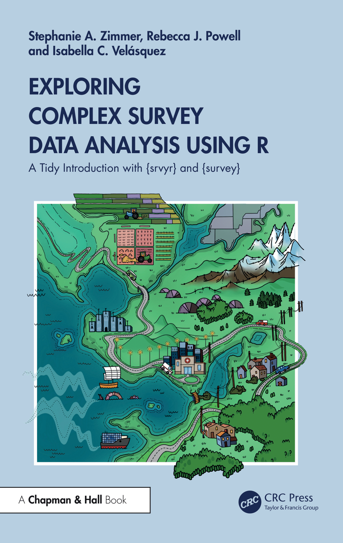
• High level overview of survey process
• Comparison of syntax between {dplyr} and {srvyr}
• How to read survey documentation
• Descriptive analysis, statistical testing, and modeling
• Publication ready tables and figures accounting for error
• Creating the survey design object
• Analysis examples using real world data

• Assume that weights are already on the dataset
• Does not include how to create weights

Where to find our book

Print copies:

• Routledge
• Your local bookstore
• Amazon

Online version:

• https://tidy-survey-r.github.io/tidy-survey-book/

Python package: svy

svy: a Python Package for the Design, Analysis, and Reporting of Complex Survey Data

• Designed to provide equivalent design-based inference to R’s survey package
  • Complex survey design (strata, clusters, weights)
  • Design-based estimation with valid standard errors
  • Replication methods (BRR, bootstrap, jackknife)
  • Small Area Estimation (area- and unit-level models)
  • Explicit, inspectable, reproducible outputs
  • Integration with Polars, NumPy, SciPy, and JAX-based tooling

Link to documentation: https://svylab.com/docs/svy/

References

• Freedman Ellis, Greg, and Ben Schneider. 2024. srvyr: ’dplyr’-Like Syntax for Summary Statistics of Survey Data. http://gdfe.co/srvyr/.
• Lumley, Thomas. 2010. Complex Surveys: A Guide to Analysis Using R. John Wiley & Sons. https://r-survey.r-forge.r-project.org/survey/.
• Zimmer, S. A., Powell, R. J., & Velásquez, I. C. (2024). Exploring Complex Survey Data Analysis Using R: A Tidy Introduction with {srvyr} and {survey}. Chapman & Hall: CRC Press. https://tidy-survey-r.github.io/tidy-survey-book/

Q & A

• Contact info will be shared in the chat

Extra material

R, SAS, & SUDAAN capabilities

Feature	R {survey} package	SAS survey procs	SUDAAN procs
Descriptive (out of the box)	mean, total, proportion, percentage, quantile, ratio, variance, correlation	mean, total, proportion, percentage, geometric mean, quantile, ratio, variance	mean, total, proportion, percentage, geometric mean, quantile, ratio, variance, correlation
Custom descriptive functions	Yes, but must use delta method	No method in docs	Yes, through vargen proc
Testing	means, proportions, quantiles, assocation, GOF	means, proportions, assocation, GOF	means, proportions, assocation, GOF
Design effects	Not for quantiles, variances, or correlations	Only for proportions	All ests
Imputation	None	Hot-deck, approximate Bayesian bootstrap, fully efficient fractional, two-stage fully efficient fractional, fractional hot-deck	Weighted sequential hot deck, cell mean, regression-based (linear and logistic)
Weighting	Post-stratification in estimation, calibration (linear, raking, logit)	Post-stratification in estimation	Post-stratification in estimation, calibration: nonresponse and post-stratification (WTADJUST), Using variables only known for respondents in models (WTADJX)
Modeling	Linear, Logistic, Cox proportional hazards, Kaplan-Meier, Multinomial, Poisson, Log-linear	Linear, Logistic, Cox proportional hazards	Linear, Logistic, Cox proportional hazards, Kaplan-Meier, Multinomial, Poisson-like count

• R comparison only includes survey and srvyr packages, not other R packages
• Bold entries in rows with bold indicate differences since there are some long lists
• R and SUDAAN allow for more customization than SAS but harder in R (need calculus to do delta method)
• R is only software doing testing of quantiles - some papers on how to do in others but requires custom macros
• SAS doesn’t broadly do design effects but there are some macros out there. We won’t go into details but more types of design effects in SUDAAN than R
• Imputation is done in other R packages
• Weighting: all allow post-stratification while doing analysis, common in health research. Other packages in R do more than survey package
• SAS does sample selection