Categorical Survey of
Complex Survey Data in R

A Hands-On Course

Rebecca J. Powell

Fors Marsh

Isabella C. Velásquez

Posit

2025-11-21

Introduction

About Us

Rebecca Powell

Fors Marsh

Isabella Velásquez

Posit

Each of us give a brief intro on our experience/background

Background

• This tutorial largely builds off our book written with Stephanie Zimmer (RTI): Exploring Complex Survey Data Analysis Using R
  • https://tidy-survey-r.github.io/site/
• The book covers additional topics outside this tutorial including:
  • Overview of survey process
  • Working with continuous variables
  • Communication of results (tables and plots)
  • Reproducible research best practices
• Not covered
  • Weighting (calibration, post-stratification, raking, etc.)
  • Survival analysis
  • Nonlinear models

Motivation

• We are R users who work with survey data regularly
• We wanted to share knowledge with
  • R users who may be inaccurately analyzing survey data
  • SAS/SUDAAN/Stata users who may not know about the capabilities of R
• {srvyr} package developed using tidyverse style syntax

Prerequisites

Tidyverse familiarity

• Selecting a set of variables (select(starts_with("TOT")))
• Creating new variables with mutate()
• Summarizing data with summarize()
• Using group_by() with summarize() to create group summaries

Overview of tutorial

• At the end of this tutorial, you should be able to
  • Calculate point estimates and their standard errors with survey data
    • Proportions, totals, and counts
  • Perform chi-squared tests
  • Conduct basic logistic regression
  • Specify a survey design in R to create a survey object

Roadmap for today

• Getting started
• Descriptive analysis
• Statistical testing
• Modeling
• Sampling design

Logistics

• We will be using Posit Cloud for exercises
• All materials are found at:
  • https://tidy-survey-r.github.io/mapor-2025-short-course/full-slide-deck.html (Site)
  • https://github.com/tidy-survey-r/mapor-2025-short-course/ (Source)

Warm Up

Welcome to the Towny Data

• We’ll be using the towny data for warm-up exercises
• Available in the {gt} package

Welcome to the Towny Data

library(tidyverse)
library(gt)
glimpse(towny)

Rows: 414
Columns: 25
$ name                     <chr> "Addington Highlands", "Adelaide Metcalfe"…
$ website                  <chr> "https://addingtonhighlands.ca", "https://…
$ status                   <chr> "lower-tier", "lower-tier", "lower-tier", …
$ csd_type                 <chr> "township", "township", "township", "towns…
$ census_div               <chr> "Lennox and Addington", "Middlesex", "Simc…
$ latitude                 <dbl> 45.00000, 42.95000, 44.13333, 45.52917, 43…
$ longitude                <dbl> -77.25000, -81.70000, -79.93333, -76.89694…
$ land_area_km2            <dbl> 1293.99, 331.11, 371.53, 519.59, 66.64, 11…
$ population_1996          <int> 2429, 3128, 9359, 2837, 64430, 1027, 8315,…
$ population_2001          <int> 2402, 3149, 10082, 2824, 73753, 956, 8593,…
$ population_2006          <int> 2512, 3135, 10695, 2716, 90167, 958, 8654,…
$ population_2011          <int> 2517, 3028, 10603, 2844, 109600, 864, 9196…
$ population_2016          <int> 2318, 2990, 10975, 2935, 119677, 969, 9680…
$ population_2021          <int> 2534, 3011, 10989, 2995, 126666, 954, 9949…
$ density_1996             <dbl> 1.88, 9.45, 25.19, 5.46, 966.84, 8.81, 21.…
$ density_2001             <dbl> 1.86, 9.51, 27.14, 5.44, 1106.74, 8.20, 21…
$ density_2006             <dbl> 1.94, 9.47, 28.79, 5.23, 1353.05, 8.22, 22…
$ density_2011             <dbl> 1.95, 9.14, 28.54, 5.47, 1644.66, 7.41, 23…
$ density_2016             <dbl> 1.79, 9.03, 29.54, 5.65, 1795.87, 8.31, 24…
$ density_2021             <dbl> 1.96, 9.09, 29.58, 5.76, 1900.75, 8.18, 25…
$ pop_change_1996_2001_pct <dbl> -0.0111, 0.0067, 0.0773, -0.0046, 0.1447, …
$ pop_change_2001_2006_pct <dbl> 0.0458, -0.0044, 0.0608, -0.0382, 0.2226, …
$ pop_change_2006_2011_pct <dbl> 0.0020, -0.0341, -0.0086, 0.0471, 0.2155, …
$ pop_change_2011_2016_pct <dbl> -0.0791, -0.0125, 0.0351, 0.0320, 0.0919, …
$ pop_change_2016_2021_pct <dbl> 0.0932, 0.0070, 0.0013, 0.0204, 0.0584, -0…

Posit Cloud

• We will be using Posit Cloud for exercises
• Posit Cloud has the same features and appearance as RStudio for ease of use
• Access the project and files Posit Cloud (requires a free account)
• Create a permanent copy if you want to save your work and access later

Your Turn

• Go to bit.ly/MAPOR-2025-short-course
• Open 02-getting-started_exercises.qmd

Packages

R Packages for Survey Analysis

• {survey} package first on CRAN in 2003
  • descriptive analysis
  • statistical testing
  • modeling
  • weighting
• {srvyr} package first on CRAN in 2016
  • “wrapper” for {survey} with {tidyverse}-style syntax
  • only descriptive analysis

Install Packages

Install packages for data wrangling and survey analysis:

install.packages(c("tidyverse", "survey", "srvyr"))

Install {srvyrexploR} to access the survey data for today’s short course:

install.packages("pak")
pak::pak("tidy-survey-r/srvyrexploR")

Load the packages:

library(tidyverse)
library(survey)
library(srvyr)
library(srvyrexploR)

Note: Installation of packages is already done for you on Posit Cloud

Data and Design Object

American National Election Studies (ANES) 2024

• Stored as anes_2024 in {srvyrexploR}
• Pre- and post-election surveys fielded almost every 2 years since 1948
• Topics include voter registration status, candidate preference, opinions on country and government, party and ideology affiliation, opinions on policy, news sources, and more
• Collaboration of Stanford, University of Michigan - funding by the National Science Foundation
• Target Population: US citizens, 18 and older living in US
• Mode: In-Person, Web, videoconference, Paper, or telephone
• Sample Information: Pseudo-strata and pseudo-cluster included for variance estimation

https://electionstudies.org/

American National Election Studies (ANES) 2024

anes_2024 %>%
  select(-matches("^V\\d")) %>%
  glimpse()

Rows: 4,764
Columns: 29
$ CaseID                  <dbl> 140001, 140002, 140003, 140004, 140005, 140…
$ Weight                  <dbl> 0.7809746, 2.5070750, 0.8144009, 0.2634901,…
$ Stratum                 <dbl> 90, 107, 122, 110, 104, 118, 88, 118, 122, …
$ VarUnit                 <dbl> 2, 2, 1, 2, 1, 2, 1, 2, 2, 1, 1, 2, 2, 2, 1…
$ InterviewMode_Pre       <fct> 2. Internet (WEB), 2. Internet (WEB), 2. In…
$ InterviewMode_Post      <fct> 2. Internet (WEB), 2. Internet (WEB), 2. In…
$ CampaignInterest        <fct> 1. Very much interested, 3. Not much intere…
$ VotedPres2020           <fct> "1. Yes, voted", "2. No, didn't vote", "1. …
$ VotedPres2020_selection <fct> 2. Donald Trump, NA, 1. Joe Biden, NA, NA, …
$ PartyID                 <fct> 7. Strong Republican, 4. Independent, 1. St…
$ TrustGovernment         <fct> 5. Never, 5. Never, 4. Some of the time, 4.…
$ TrustPeople             <fct> 3. About half the time, 3. About half the t…
$ Age                     <dbl> 50, 41, 44, 45, 80, 75, 41, 49, 45, 41, 59,…
$ Education               <dbl> 13, 10, 10, 11, 16, 10, 11, 10, 9, 9, 9, 9,…
$ RaceEth                 <fct> "3. Hispanic", "4. Asian or Native Hawaiian…
$ Sex                     <fct> 1. Male, 2. Female, 2. Female, 1. Male, 1. …
$ Income                  <fct> "27. $175,000-249,999", "26. $150,000-174,9…
$ EarlyVote               <fct> 2. Have not voted, 2. Have not voted, 2. Ha…
$ EarlyVoteGeneral        <fct> NA, NA, NA, NA, NA, NA, NA, NA, NA, NA, "2.…
$ Post_Vote24             <fct> "4. I am sure I voted", "3. I usually vote,…
$ Pre_VotePres24          <fct> NA, NA, NA, NA, NA, NA, NA, NA, NA, NA, NA,…
$ Post_VotePres24         <fct> "1. Yes, voted for President", NA, "1. Yes,…
$ VotedPres2024_selection <fct> 2. Donald Trump, NA, 1. Kamala Harris, NA, …
$ AgeGroup                <fct> 50-59, 40-49, 40-49, 40-49, 70 or older, 70…
$ EducationGroup          <fct> Bachelor's, Post HS, Post HS, Post HS, Grad…
$ Income7                 <fct> "$125k or more", "$125k or more", "$100k to…
$ EarlyVote2024           <chr> "2. Have not voted", "2. Have not voted", "…
$ Voted2024               <chr> "Yes", "No", "Yes", "No", "Yes", "No", "Yes…
$ VotedPres2024           <chr> "Yes", "No", "Yes", "No", "Yes", "No", "Yes…

Design Object

• Backbone for survey analysis
• Specify the sampling design, weights, and other necessary information to account for errors in the data
• Survey analysis and inference should be performed with the survey design objects, not the original survey data
• We will be covering survey design in more detail later!

American National Election Studies Design Object

anes_des <- anes_2024 %>%
  mutate(Weight = V240108b / sum(V240108b) * 232449541) %>%
  as_survey_design(
    weights = Weight,
    strata = V240108d,
    ids = V240108c,
    nest = TRUE
  )

American National Election Studies Design Object

anes_des

Stratified 1 - level Cluster Sampling design (with replacement)
With (1934) clusters.
Called via srvyr
Sampling variables:
  - ids: V240108c 
  - strata: V240108d 
  - weights: Weight 
Data variables: 
  - CaseID (dbl), Weight (dbl), Stratum (dbl), VarUnit (dbl),
    InterviewMode_Pre (fct), InterviewMode_Post (fct), CampaignInterest
    (fct), VotedPres2020 (fct), VotedPres2020_selection (fct), PartyID
    (fct), TrustGovernment (fct), TrustPeople (fct), Age (dbl), Education
    (dbl), RaceEth (fct), Sex (fct), Income (fct), EarlyVote (fct),
    EarlyVoteGeneral (fct), Post_Vote24 (fct), Pre_VotePres24 (fct),
    Post_VotePres24 (fct), VotedPres2024_selection (fct), AgeGroup (fct),
    EducationGroup (fct), Income7 (fct), EarlyVote2024 (chr), Voted2024
    (chr), VotedPres2024 (chr), V240001 (dbl), V240002a (hvn_lbll), V240002b
    (hvn_lbll), V240108b (dbl), V240108d (dbl), V240108c (dbl), V241005
    (hvn_lbll), V241103 (hvn_lbll), V241104 (hvn_lbll), V241038 (hvn_lbll),
    V241221 (hvn_lbll), V241222 (hvn_lbll), V241223 (hvn_lbll), V241227x
    (hvn_lbll), V241229 (hvn_lbll), V241234 (hvn_lbll), V241458x (hvn_lbll),
    V241463 (hvn_lbll), V241499 (hvn_lbll), V241501x (hvn_lbll), V241550
    (hvn_lbll), V241566x (hvn_lbll), V242065 (hvn_lbll), V241035 (hvn_lbll),
    V241036 (hvn_lbll), V241037 (hvn_lbll), V242051 (hvn_lbll), V242095x
    (hvn_lbll), V242066 (hvn_lbll), V241039 (hvn_lbll), V242067 (hvn_lbll),
    V242096x (hvn_lbll)

Comparison of {dplyr} and {srvyr} Functions

Why use {srvyr} over {survey}?

• Use the pipe function %>% or |>
• Ability to use tidy selection
• Functions follow snake_case convention

Apply {dplyr} functions to survey objects

• A few functions in {srvyr} have counterparts in {dplyr}
  • dplyr::summarize() and srvyr::summarize()
  • dplyr::group_by() and srvyr::group_by()
• Based on the object class, R will recognize which package to use

Using summarize() to calculate mean and median

Tibble:

towny %>%
  summarize(
    area_mean = mean(land_area_km2, na.rm=TRUE)
  )

# A tibble: 1 × 1
  area_mean
      <dbl>
1      373.

Using summarize() to calculate mean and median

Survey object:

anes_des %>%
  summarize(
    age_mean = survey_mean(Age, na.rm=TRUE),
  )

# A tibble: 1 × 2
  age_mean age_mean_se
     <dbl>       <dbl>
1     48.5       0.445

Using {dplyr} functions

Tibble:

towny %>%
  filter(csd_type == "township") %>%
  select(csd_type, name)

# A tibble: 195 × 2
   csd_type name                  
   <chr>    <chr>                 
 1 township Addington Highlands   
 2 township Adelaide Metcalfe     
 3 township Adjala-Tosorontio     
 4 township Admaston/Bromley      
 5 township Alberton              
 6 township Alfred and Plantagenet
 7 township Algonquin Highlands   
 8 township Alnwick/Haldimand     
 9 township Amaranth              
10 township The Archipelago       
# ℹ 185 more rows

Using {dplyr} functions

Survey object:

anes_des %>%
  filter(EducationGroup == "Graduate") %>%
  select(Sex)

Stratified 1 - level Cluster Sampling design (with replacement)
With (492) clusters.
Called via srvyr
Sampling variables:
  - ids: V240108c 
  - strata: V240108d 
  - weights: Weight 
Data variables: 
  - Sex (fct)

Grouping

Tibble:

towny %>%
  group_by(csd_type) %>%
  summarize(area_mean = mean(land_area_km2))

# A tibble: 5 × 2
  csd_type     area_mean
  <chr>            <dbl>
1 city             498. 
2 municipality     607. 
3 town             183. 
4 township         363. 
5 village           23.0

Grouping

Survey object:

anes_des %>%
  group_by(EducationGroup) %>%
  summarize(age_mean = survey_mean(Age, na.rm=TRUE))

# A tibble: 6 × 3
  EducationGroup age_mean age_mean_se
  <fct>             <dbl>       <dbl>
1 Less than HS       50.1       1.76 
2 High school        48.3       0.904
3 Post HS            48.2       0.709
4 Bachelor's         46.5       0.731
5 Graduate           51.8       0.797
6 <NA>               52.9       4.76 

Using {srvyr} functions on non-survey objects

towny %>%
  summarize(area_mean = survey_mean(land_area_km2))

Error in `summarize()`:
ℹ In argument: `area_mean = survey_mean(land_area_km2)`.
Caused by error in `cur_svy()`:
! Survey context not set

Survey Analysis Process

Overview of Survey Analysis using {srvyr} Package

1. Create a tbl_svy object (a survey object) using: as_survey_design() or as_survey_rep()

2. Subset data (if needed) using filter() (to create subpopulations)

3. Specify domains of analysis using group_by()

4. Within summarize(), specify variables to calculate, including means, totals, proportions, quantiles, and more

Descriptive Analysis

Introduction

Descriptive analyses lay the groundwork for the next steps of running statistical tests or developing models.

Calculate point estimates of…

• Unknown population parameters, such as mean.

• Uncertainty estimates, such as confidence intervals.

Types of data

• Categorical/nominal data: variables with levels or descriptions that cannot be ordered, such as the region of the country (North, South, East, and West)

• Ordinal data: variables that can be ordered, such as those from a Likert scale (strongly disagree, disagree, agree, and strongly agree)
• Discrete data: variables that are counted or measured, such as number of children
• Continuous data: variables that are measured and whose values can lie anywhere on an interval, such as income

Types of measures

• Measures of distribution describe how often an event or response occurs.
  • Count of observations with survey_count()
• Measures of central tendency find the central (or average) responses.
  • Proportions with survey_prop() and survey_total()

Overview of survey analysis using the {srvyr} package

1. Create a tbl_svy object (a survey object) using: as_survey_design() or as_survey_rep()

2. Subset data (if needed) using filter() (to create subpopulations)

3. Specify domains of analysis using group_by()

4. Specify variables to calculate, including means, totals, proportions, quantiles, and more

Counts and totals

survey_count()

• Calculate the estimated observation counts for a given variable or combination of variables
• Applied to categorical data
• Sometimes called “cross-tabulations” or “cross-tabs”
• survey_count() functions similarly to dplyr::count() in that it is NOT called within summarize()

survey_count(): syntax

survey_count(
  x,
  ...,
  wt = NULL,
  sort = FALSE,
  name = "n",
  .drop = dplyr::group_by_drop_default(x),
  vartype = c("se", "ci", "var", "cv")
)

survey_count: example

Estimate the number of U.S. adults (18+) living in the continental United States using ANES data:

anes_des %>%
  survey_count()

# A tibble: 1 × 2
           n     n_se
       <dbl>    <dbl>
1 232449541. 5069171.

survey_count: subgroup example

Calculate the weighted estimate of respondents by voting status in the 2024 election:

anes_des %>%
  survey_count(
    Voted2024, 
    name = "N"
    )

# A tibble: 2 × 3
  Voted2024          N     N_se
  <chr>          <dbl>    <dbl>
1 No         49326605. 2859120.
2 Yes       183122936. 4071109.

survey_total(): syntax

• The survey_total() function is analogous to sum()
• survey_total() must be used within summarize()
• If used with no x-variable, survey_total() calculates a population count estimate within summarize()

survey_total(): example

Estimate the number of U.S. adults (18+) living in the continental United States using ANES data:

anes_des %>%
  summarize(
    survey_total()
  )

# A tibble: 1 × 2
        coef    `_se`
       <dbl>    <dbl>
1 232449541. 5069171.

unweighted()

• Sometimes, it is helpful to calculate an unweighted estimate of a given variable
• unweighted() does not extrapolate to a population estimate
• Used in conjunction with any {dplyr} functions

unweighted(): example

Calculate the weighted and unweighted number of survey respondents:

anes_des %>%
  summarize(
    n_unweighted = unweighted(n()),
    n_weighted = survey_total()
  )

# A tibble: 1 × 3
  n_unweighted n_weighted n_weighted_se
         <int>      <dbl>         <dbl>
1         4764 232449541.      5069171.

Proportions

survey_prop()

• Calculate the estimated observation counts for a given variable or combination of variables
• survey_prop() to categorical data
• Must be called within summarize()

survey_prop(): syntax

survey_prop(
  na.rm = FALSE,
  vartype = c("se", "ci", "var", "cv"),
  level = 0.95,
  proportion = TRUE,
  prop_method =
    c("logit", "likelihood", "asin", "beta", "mean", "xlogit"),
  deff = FALSE,
  df = NULL
)

survey_prop(): one variable proportion example

Calculate the proportion of respondents by voting status in the 2024 election:

anes_des %>%
  group_by(Voted2024) %>%
  summarize(p = survey_prop())

# A tibble: 2 × 3
  Voted2024     p   p_se
  <chr>     <dbl>  <dbl>
1 No        0.212 0.0102
2 Yes       0.788 0.0102

survey_prop(): conditional proportions example

Calculate the proportion of whether someone voted by campaign interest:

anes_des %>%
  group_by(Voted2024, CampaignInterest) %>%
  summarize(p = survey_prop())

# A tibble: 7 × 4
# Groups:   Voted2024 [2]
  Voted2024 CampaignInterest              p    p_se
  <chr>     <fct>                     <dbl>   <dbl>
1 No        1. Very much interested 0.147   0.0162 
2 No        2. Somewhat interested  0.485   0.0244 
3 No        3. Not much interested  0.367   0.0225 
4 No        <NA>                    0.00170 0.00170
5 Yes       1. Very much interested 0.537   0.0109 
6 Yes       2. Somewhat interested  0.367   0.0111 
7 Yes       3. Not much interested  0.0956  0.00647

survey_prop(): joint proportions example

Calculate the joint proportions for each variable combination using interact():

anes_des %>%
  group_by(interact(Voted2024, CampaignInterest)) %>%
  summarize(p = survey_prop())

# A tibble: 7 × 4
  Voted2024 CampaignInterest               p     p_se
  <chr>     <fct>                      <dbl>    <dbl>
1 No        1. Very much interested 0.0312   0.00363 
2 No        2. Somewhat interested  0.103    0.00732 
3 No        3. Not much interested  0.0778   0.00612 
4 No        <NA>                    0.000361 0.000361
5 Yes       1. Very much interested 0.423    0.0102  
6 Yes       2. Somewhat interested  0.289    0.00970 
7 Yes       3. Not much interested  0.0753   0.00510 

Helper functions for survey analysis

filter()

• Allows for subpopulation analysis
• Use filter() to subset a survey object for analysis
• Must be done after creating the survey design object

filter(): example

Estimate the proportion of 2024 voters among respondents who voted in 2020:

anes_des %>%
  filter(VotedPres2020 == "1. Yes, voted") %>%
  group_by(Voted2024) %>%
  summarize(
    survey_prop()
  )

# A tibble: 2 × 3
  Voted2024   coef   `_se`
  <chr>      <dbl>   <dbl>
1 No        0.0770 0.00767
2 Yes       0.923  0.00767

cascade()

• The {srvyr} package has the convenient cascade() function
• Used instead of summarize()
• Creates a summary row for the estimate representing the entire population

cascade(): syntax

cascade(
  .data, 
  ..., 
  .fill = NA, 
  .fill_level_top = FALSE, 
  .groupings = NULL
)

cascade(): example

Estimate the share of respondents who did and did not vote in the 2024 election, then demonstrate the features of cascade():

anes_des %>%
  group_by(Voted2024) %>%
  cascade(prop = survey_prop())

# A tibble: 3 × 3
  Voted2024  prop  prop_se
  <chr>     <dbl>    <dbl>
1 No        0.212 1.02e- 2
2 Yes       0.788 1.02e- 2
3 <NA>      1.000 9.68e-18

cascade(): example

Give the summary row a better name with .fill:

anes_des %>%
  group_by(Voted2024) %>%
  cascade(prop = survey_prop(),
          .fill = "All")

# A tibble: 3 × 3
  Voted2024  prop  prop_se
  <chr>     <dbl>    <dbl>
1 All       1.000 9.68e-18
2 No        0.212 1.02e- 2
3 Yes       0.788 1.02e- 2

cascade(): example

Move the summary row to the top with .fill_level_top = TRUE:

anes_des %>%
  group_by(Voted2024) %>%
  cascade(prop = survey_prop(),
          .fill = "All",
          .fill_level_top = TRUE)

# A tibble: 3 × 3
  Voted2024  prop  prop_se
  <chr>     <dbl>    <dbl>
1 All       1.000 9.68e-18
2 No        0.212 1.02e- 2
3 Yes       0.788 1.02e- 2

Your Turn

• Go to bit.ly/MAPOR-2025-short-course
• Open 03-descriptive-exercises.qmd

Chi-square tests

Chi-square tests

• Compare multiple proportions to see if they are statistically different from each other

• Different types:
  • Goodness-of-fit tests compare observed data to expected data
  • Tests of independence compare two types of observed data to see if there is a relationship
  • Tests of homogeneity compare two distributions to see if they match

Chi-square syntax

There are two functions that we use to compare proportions:

• svygofchisq(): For goodness-of-fit tests
• svychisq(): For tests of independence and homogeneity

Syntax for goodness-of-fit tests

svygofchisq(
  formula,
  p,
  design,
  na.rm = TRUE,
  ...
)

Syntax for tests of independence and homogeneity

svychisq(
  formula,
  design,
  statistic = c(
    "F", "Chisq", "Wald", "adjWald",
    "lincom", "saddlepoint"
  ),
  na.rm = TRUE,
  ...
)

Example
goodness-of-fit test

Example: goodness-of-fit test

• Let’s check to see if the education levels from the ANES match the levels from the ACS
• Here is the education breakdown from the ACS in 2024
  • 10% had less than a high school degree
  • 27% had a high school degree
  • 29% had some college or an associate’s degree
  • 34% had a bachelor’s degree or higher

Example: goodness-of-fit test

• Let’s check to see if the education levels from the ANES match the levels from the ACS
• Here is the education breakdown from our survey data

anes_des %>%
  drop_na(EducationGroup) %>%
  group_by(EducationGroup) %>%
  summarize(p = survey_mean())

# A tibble: 5 × 3
  EducationGroup      p    p_se
  <fct>           <dbl>   <dbl>
1 Less than HS   0.0824 0.00673
2 High school    0.270  0.00948
3 Post HS        0.302  0.00923
4 Bachelor's     0.213  0.00816
5 Graduate       0.132  0.00633

• Use drop_na() to first remove any missing data from the Education variable
• Use group_by() and summarize() to get the proportions by Education level

Example: goodness-of-fit test

Let’s collapse Bachelor’s and Graduate degrees into a single category for comparison.

anes_des_educ <- anes_des %>%
  mutate(
    Education2 =
      fct_collapse(EducationGroup,
        "Bachelor or Higher" = c("Bachelor's", "Graduate")
      )
  )

Example: goodness-of-fit test

anes_des_educ %>%
  drop_na(Education2) %>%
  group_by(Education2) %>%
  summarize(p = survey_mean())

# A tibble: 4 × 3
  Education2              p    p_se
  <fct>               <dbl>   <dbl>
1 Less than HS       0.0824 0.00673
2 High school        0.270  0.00948
3 Post HS            0.302  0.00923
4 Bachelor or Higher 0.346  0.00914

Example: goodness-of-fit test

Test to see if the ANES education matches the population percentages

anes_des_educ %>%
  svygofchisq(
    ~Education2,
    p = c(0.10, 0.27, 0.29, 0.34),
    na.rm = TRUE
  )

Error in UseMethod("svytotal", design): no applicable method for 'svytotal' applied to an object of class "formula"

• as design argument is the second argument, dot notation is needed

Dot notation

Dot notation

Let’s walk through an example using the towny data.

towny

# A tibble: 414 × 25
   name   website status csd_type census_div latitude longitude land_area_km2
   <chr>  <chr>   <chr>  <chr>    <chr>         <dbl>     <dbl>         <dbl>
 1 Addin… https:… lower… township Lennox an…     45       -77.2        1294. 
 2 Adela… https:… lower… township Middlesex      43.0     -81.7         331. 
 3 Adjal… https:… lower… township Simcoe         44.1     -79.9         372. 
 4 Admas… https:… lower… township Renfrew        45.5     -76.9         520. 
 5 Ajax   https:… lower… town     Durham         43.9     -79.0          66.6
 6 Alber… https:… singl… township Rainy Riv…     48.6     -93.5         117. 
 7 Alfre… https:… lower… township Prescott …     45.6     -74.9         392. 
 8 Algon… https:… lower… township Haliburton     45.4     -78.8        1000. 
 9 Alnwi… https:… lower… township Northumbe…     44.1     -78.0         398. 
10 Amara… https:… lower… township Dufferin       44.0     -80.2         265. 
# ℹ 404 more rows
# ℹ 17 more variables: population_1996 <int>, population_2001 <int>,
#   population_2006 <int>, population_2011 <int>, population_2016 <int>,
#   population_2021 <int>, density_1996 <dbl>, density_2001 <dbl>,
#   density_2006 <dbl>, density_2011 <dbl>, density_2016 <dbl>,
#   density_2021 <dbl>, pop_change_1996_2001_pct <dbl>,
#   pop_change_2001_2006_pct <dbl>, pop_change_2006_2011_pct <dbl>, …

Dot notation

Using the towny data, let’s filter to only cities.

filter(towny, csd_type == "city")

# A tibble: 52 × 25
   name   website status csd_type census_div latitude longitude land_area_km2
   <chr>  <chr>   <chr>  <chr>    <chr>         <dbl>     <dbl>         <dbl>
 1 Barrie https:… singl… city     Simcoe         44.4     -79.7          99.0
 2 Belle… https:… singl… city     Hastings       44.2     -77.4         247. 
 3 Bramp… https:… lower… city     Peel           43.7     -79.8         266. 
 4 Brant  https:… singl… city     Brant          43.1     -80.4         818. 
 5 Brant… https:… singl… city     Brant          43.1     -80.3          98.6
 6 Brock… https:… singl… city     Leeds and…     44.6     -75.7          20.9
 7 Burli… https:… lower… city     Halton         43.4     -79.8         186. 
 8 Cambr… https:… lower… city     Waterloo       43.4     -80.3         113. 
 9 Clare… https:… lower… city     Prescott …     45.5     -75.2         297. 
10 Cornw… https:… singl… city     Stormont,…     45.0     -74.7          61.5
# ℹ 42 more rows
# ℹ 17 more variables: population_1996 <int>, population_2001 <int>,
#   population_2006 <int>, population_2011 <int>, population_2016 <int>,
#   population_2021 <int>, density_1996 <dbl>, density_2001 <dbl>,
#   density_2006 <dbl>, density_2011 <dbl>, density_2016 <dbl>,
#   density_2021 <dbl>, pop_change_1996_2001_pct <dbl>,
#   pop_change_2001_2006_pct <dbl>, pop_change_2006_2011_pct <dbl>, …

Dot notation

Using the towny data, let’s filter to only cities.

filter(towny, csd_type == "city")
towny %>% filter(csd_type == "city")

# A tibble: 52 × 25
   name   website status csd_type census_div latitude longitude land_area_km2
   <chr>  <chr>   <chr>  <chr>    <chr>         <dbl>     <dbl>         <dbl>
 1 Barrie https:… singl… city     Simcoe         44.4     -79.7          99.0
 2 Belle… https:… singl… city     Hastings       44.2     -77.4         247. 
 3 Bramp… https:… lower… city     Peel           43.7     -79.8         266. 
 4 Brant  https:… singl… city     Brant          43.1     -80.4         818. 
 5 Brant… https:… singl… city     Brant          43.1     -80.3          98.6
 6 Brock… https:… singl… city     Leeds and…     44.6     -75.7          20.9
 7 Burli… https:… lower… city     Halton         43.4     -79.8         186. 
 8 Cambr… https:… lower… city     Waterloo       43.4     -80.3         113. 
 9 Clare… https:… lower… city     Prescott …     45.5     -75.2         297. 
10 Cornw… https:… singl… city     Stormont,…     45.0     -74.7          61.5
# ℹ 42 more rows
# ℹ 17 more variables: population_1996 <int>, population_2001 <int>,
#   population_2006 <int>, population_2011 <int>, population_2016 <int>,
#   population_2021 <int>, density_1996 <dbl>, density_2001 <dbl>,
#   density_2006 <dbl>, density_2011 <dbl>, density_2016 <dbl>,
#   density_2021 <dbl>, pop_change_1996_2001_pct <dbl>,
#   pop_change_2001_2006_pct <dbl>, pop_change_2006_2011_pct <dbl>, …

Dot notation

Using the towny data, let’s filter to only cities.

filter(towny, csd_type == "city")
towny %>% filter(csd_type == "city")
towny %>% filter(., csd_type == "city")

# A tibble: 52 × 25
   name   website status csd_type census_div latitude longitude land_area_km2
   <chr>  <chr>   <chr>  <chr>    <chr>         <dbl>     <dbl>         <dbl>
 1 Barrie https:… singl… city     Simcoe         44.4     -79.7          99.0
 2 Belle… https:… singl… city     Hastings       44.2     -77.4         247. 
 3 Bramp… https:… lower… city     Peel           43.7     -79.8         266. 
 4 Brant  https:… singl… city     Brant          43.1     -80.4         818. 
 5 Brant… https:… singl… city     Brant          43.1     -80.3          98.6
 6 Brock… https:… singl… city     Leeds and…     44.6     -75.7          20.9
 7 Burli… https:… lower… city     Halton         43.4     -79.8         186. 
 8 Cambr… https:… lower… city     Waterloo       43.4     -80.3         113. 
 9 Clare… https:… lower… city     Prescott …     45.5     -75.2         297. 
10 Cornw… https:… singl… city     Stormont,…     45.0     -74.7          61.5
# ℹ 42 more rows
# ℹ 17 more variables: population_1996 <int>, population_2001 <int>,
#   population_2006 <int>, population_2011 <int>, population_2016 <int>,
#   population_2021 <int>, density_1996 <dbl>, density_2001 <dbl>,
#   density_2006 <dbl>, density_2011 <dbl>, density_2016 <dbl>,
#   density_2021 <dbl>, pop_change_1996_2001_pct <dbl>,
#   pop_change_2001_2006_pct <dbl>, pop_change_2006_2011_pct <dbl>, …

Dot notation

Using the towny data, let’s filter to only cities.

filter(towny, csd_type == "city")
towny %>% filter(csd_type == "city")
towny %>% filter(., csd_type == "city")
towny %>% filter(.data = ., csd_type == "city")

# A tibble: 52 × 25
   name   website status csd_type census_div latitude longitude land_area_km2
   <chr>  <chr>   <chr>  <chr>    <chr>         <dbl>     <dbl>         <dbl>
 1 Barrie https:… singl… city     Simcoe         44.4     -79.7          99.0
 2 Belle… https:… singl… city     Hastings       44.2     -77.4         247. 
 3 Bramp… https:… lower… city     Peel           43.7     -79.8         266. 
 4 Brant  https:… singl… city     Brant          43.1     -80.4         818. 
 5 Brant… https:… singl… city     Brant          43.1     -80.3          98.6
 6 Brock… https:… singl… city     Leeds and…     44.6     -75.7          20.9
 7 Burli… https:… lower… city     Halton         43.4     -79.8         186. 
 8 Cambr… https:… lower… city     Waterloo       43.4     -80.3         113. 
 9 Clare… https:… lower… city     Prescott …     45.5     -75.2         297. 
10 Cornw… https:… singl… city     Stormont,…     45.0     -74.7          61.5
# ℹ 42 more rows
# ℹ 17 more variables: population_1996 <int>, population_2001 <int>,
#   population_2006 <int>, population_2011 <int>, population_2016 <int>,
#   population_2021 <int>, density_1996 <dbl>, density_2001 <dbl>,
#   density_2006 <dbl>, density_2011 <dbl>, density_2016 <dbl>,
#   density_2021 <dbl>, pop_change_1996_2001_pct <dbl>,
#   pop_change_2001_2006_pct <dbl>, pop_change_2006_2011_pct <dbl>, …

Results: goodness-of-fit test

Test to see if the ANES education matches the population percentages

anes_des_educ %>%
  svygofchisq(
    formula = ~Education2,
    p = c(0.10, 0.27, 0.29, 0.34),
    design = .,
    na.rm = TRUE
  )

    Design-based chi-squared test for given probabilities

data:  ~Education2
X-squared = 848588, scale = 1.7316e+05, df = 2.1514e+00, p-value =
0.0983

Results: goodness-of-fit test

anes_des_educ %>%
  drop_na(Education2) %>%
  group_by(Education2) %>%
  summarize(Observed = survey_mean(vartype = "ci")) %>%
  rename(Education = Education2) %>%
  mutate(Expected = c(0.10, 0.27, 0.29, 0.34)) %>%
  select(Education, Expected, everything()) %>%
  pivot_longer(
    cols = c("Expected", "Observed"),
    names_to = "Names",
    values_to = "Proportion"
  ) %>%
  mutate(
    Observed_low = if_else(Names == "Observed", Observed_low, NA_real_),
    Observed_upp = if_else(Names == "Observed", Observed_upp, NA_real_),
    Names = if_else(Names == "Observed",
      "ANES (observed)", "ACS (expected)"
    )
  ) %>%
  ggplot(aes(x = Education, y = Proportion, color = Names)) +
  geom_point(alpha = 0.75, size = 2) +
  geom_errorbar(aes(ymin = Observed_low, ymax = Observed_upp),
    width = 0.25
  ) +
  theme_bw() +
  scale_color_manual(name = "Type", values = c("#ff8484", "#0b3954")) +
  theme(legend.position = "bottom", legend.title = element_blank())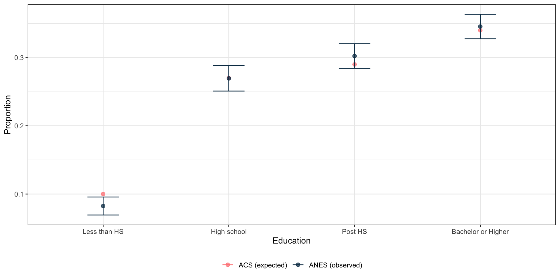

Example
test of independence

Example: test of independence

ANES asked respondents two questions about trust:

• Question text: “How often can you trust the federal government to do what is right?”
• Question text: “How often can you trust other people?”

Run a test of independence to see if there is a relationship between these two questions.

Example: test of independence

Run a test of independence to see if there is a relationship between these two questions.

anes_des %>%
  svychisq(
    formula = ~ TrustGovernment + TrustPeople,
    design = .,
    statistic = "Wald",
    na.rm = TRUE
  )

    Design-based Wald test of association

data:  NextMethod()
F = 13.611, ndf = 16, ddf = 1803, p-value < 2.2e-16

• Null Hypothesis: Independent (no relationship)
• Alt Hypothesis: Not Independent (relationship)

p-value > 0.05, so there is a relationship between these two variables

Example: test of independence

anes_des %>%
  drop_na(TrustPeople, TrustGovernment) %>%
  group_by(TrustPeople, TrustGovernment) %>%
  summarize(
    Observed = round(survey_mean(vartype = "ci"), 3),
    .groups = "drop"
  ) %>%
  mutate(prop = paste0(
    Observed, " (", Observed_low, ", ",
    Observed_upp, ")"
  )) %>%
  select(TrustGovernment, TrustPeople, prop) %>%
  pivot_wider(names_from = TrustPeople, values_from = prop) %>%
  gt(rowname_col = "TrustGovernment") %>%
  tab_stubhead(label = "Trust in Government") %>%
  tab_spanner(
    label = "Trust in People",
    columns = everything()
  ) %>%
  tab_options(page.orientation = "landscape")

Trust in Government	Trust in People
	1. Always	2. Most of the time	3. About half the time	4. Some of the time	5. Never
1. Always	0.182 (0.011, 0.352)	0.011 (0.003, 0.018)	0.009 (0.001, 0.018)	0.009 (0.003, 0.014)	0.034 (-0.001, 0.07)
2. Most of the time	0.219 (0.11, 0.328)	0.177 (0.157, 0.198)	0.09 (0.069, 0.111)	0.103 (0.077, 0.128)	0.036 (0.007, 0.065)
3. About half the time	0.228 (0.043, 0.414)	0.303 (0.273, 0.334)	0.37 (0.331, 0.41)	0.198 (0.165, 0.23)	0.11 (0.061, 0.158)
4. Some of the time	0.162 (0.046, 0.279)	0.417 (0.385, 0.449)	0.383 (0.348, 0.418)	0.509 (0.465, 0.553)	0.327 (0.231, 0.423)
5. Never	0.208 (0.069, 0.347)	0.091 (0.074, 0.109)	0.147 (0.121, 0.173)	0.182 (0.151, 0.212)	0.493 (0.399, 0.587)

Your Turn

• Go to bit.ly/MAPOR-2025-short-course
• Open 04-testing-exercises.qmd

Modeling

Introduction

• Modeling investigates the relationship between a single dependent variable and one or more independent variables.
• Logistic regression is a specific case of the generalized linear model (GLM).
• Logistic regression is used to model binary outcomes, such as whether or not someone voted.

Introduction

Assumptions in logistic regression using survey data include:

• The outcome variable has two levels
• There is a linear relationship between the independent variables and the log odds (the equation for the logit function)
• The residuals are homoscedastic; that is, the error term is the same across all values of independent variables

svyglm: syntax

des_obj %>%
  svyglm(
    formula = outcomevar ~ x1 + x2 + x3,
    design = .,
    na.action = na.omit,
    df.resid = NULL,
    family = quasibinomial
  )

svyglm: example

Model whether a person usually trusts the government based on who they voted for in 2024¹:

1. Create a binary trust variable by grouping ‘Always’ and ‘Most of the time’ into one category, and all remaining responses into the other.

anes_des_der <- anes_des %>%
  mutate(TrustGovernmentUsually = case_when(
    is.na(TrustGovernment) ~ NA,
    TRUE ~ TrustGovernment %in% c("1. Always", "2. Most of the time")
  ))

1. https://electionstudies.org/data-center/20204time-series-study/

svyglm: example

2. Summarize the data:

anes_des_summary <-
  anes_des_der %>%
  group_by(VotedPres2024_selection) %>%
  summarize(pct_trust = survey_mean(
    TrustGovernmentUsually,
    na.rm = TRUE,
    proportion = TRUE,
    vartype = "ci"),
    .groups = "drop"
    ) %>%
  filter(complete.cases(.))

svyglm: example

3. Plot the summary of the data:

anes_des_summary %>%
  ggplot(aes(
    x = VotedPres2024_selection, y = pct_trust,
    fill = VotedPres2024_selection
  )) +
  geom_bar(stat = "identity") +
  geom_errorbar(aes(ymin = pct_trust_low, ymax = pct_trust_upp),
    width = .2
  ) +
  scale_fill_manual(values = c("#0b3954", "#bfd7ea", "#8d6b94")) +
  xlab("Election choice (2020)") +
  ylab("Usually trust the government") +
  scale_y_continuous(labels = scales::percent) +
  guides(fill = "none") +
  theme_minimal()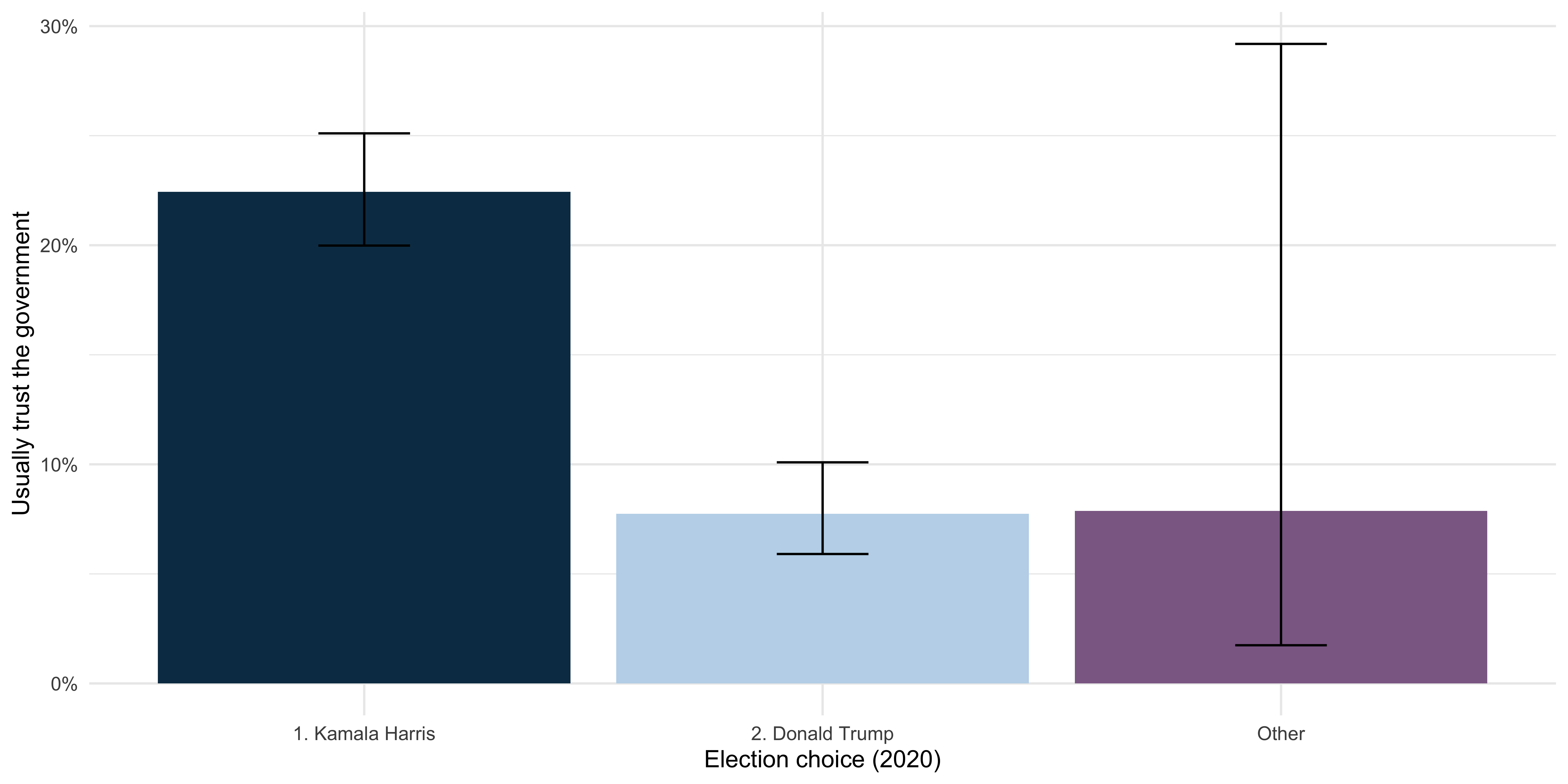

svyglm: example

4. Verify by fitting the model:

logistic_trust_vote <- anes_des_der %>%
  svyglm(
    design = .,
    formula = TrustGovernmentUsually ~ VotedPres2024_selection,
    family = quasibinomial
  )

svyglm: example

4. Verify by fitting the model:

library(broom)
library(prettyunits)
library(gt)

tidy(logistic_trust_vote) %>%
  mutate(p.value = pretty_p_value(p.value)) %>%
  gt() %>%
  fmt_number()

term	estimate	std.error	statistic	p.value
(Intercept)	−1.24	0.07	−16.54	<0.0001
VotedPres2024_selection2. Donald Trump	−1.24	0.16	−7.65	<0.0001
VotedPres2024_selectionOther	−1.22	0.75	−1.62	0.1050

svyglm: example

Result:

tidy(logistic_trust_vote) %>%
  mutate(p.value = pretty_p_value(p.value)) %>%
  gt() %>%
  fmt_number()

term	estimate	std.error	statistic	p.value
(Intercept)	−1.24	0.07	−16.54	<0.0001
VotedPres2024_selection2. Donald Trump	−1.24	0.16	−7.65	<0.0001
VotedPres2024_selectionOther	−1.22	0.75	−1.62	0.1050

1. Estimated coefficients (estimate)
2. Estimated standard errors of the coefficients (std.error)
3. p-value for each coefficient

svyglm: example

Result:

tidy(logistic_trust_vote) %>%
  mutate(p.value = pretty_p_value(p.value)) %>%
  gt() %>%
  fmt_number()

term	estimate	std.error	statistic	p.value
(Intercept)	−1.24	0.07	−16.54	<0.0001
VotedPres2024_selection2. Donald Trump	−1.24	0.16	−7.65	<0.0001
VotedPres2024_selectionOther	−1.22	0.75	−1.62	0.1050

Compared with Harris voters, Trump voters show lower levels of trust in the government.

The coefficient of -1.24 represents the increase in the log odds of usually trusting the government.

svyglm: example

To talk about odds rather than log odds, we can exponentiate the coefficients:

tidy(logistic_trust_vote, exponentiate = TRUE) %>%
  select(term, estimate) %>%
  gt() %>%
  fmt_number()

term	estimate
(Intercept)	0.29
VotedPres2024_selection2. Donald Trump	0.29
VotedPres2024_selectionOther	0.30

svyglm: example

Result:

tidy(logistic_trust_vote, exponentiate = TRUE) %>%
  select(term, estimate) %>%
  gt() %>%
  fmt_number()

term	estimate
(Intercept)	0.29
VotedPres2024_selection2. Donald Trump	0.29
VotedPres2024_selectionOther	0.30

The odds that a Trump voter usually trusts the government are about 29% of the odds for a Harris voter, who serves as the reference group.

Interaction effects

Next, examine the interaction between early voting and level of education in the model.

1. Subset to 2024 voters and create an indicator for Harris voters.

anes_des_ind <- anes_des %>%
  filter(!is.na(VotedPres2024_selection)) %>%
  mutate(VoteHarris = case_when(
    VotedPres2024_selection == "1. Kamala Harris" ~ 1,
    TRUE ~ 0
  ))

Interaction effects

2. Let’s look at the main effects of education and early voting behavior.

log_harris_main <- anes_des_ind %>%
  mutate(
    EarlyVote2024 = fct_relevel(EarlyVote2024, "2. Have not voted", after = 0)
  ) %>%
  svyglm(
    design = .,
    formula = VoteHarris ~ EarlyVote2024 + EducationGroup,
    family = quasibinomial
  )

Interaction effects

Results:

tidy(log_harris_main) %>%
  mutate(p.value = pretty_p_value(p.value)) %>%
  gt() %>%
  fmt_number()

term	estimate	std.error	statistic	p.value
(Intercept)	−0.44	0.24	−1.88	0.0604
EarlyVote20241. Have voted	0.04	0.19	0.21	0.8318
EducationGroupHigh school	0.09	0.26	0.34	0.7341
EducationGroupPost HS	0.34	0.25	1.38	0.1668
EducationGroupBachelor's	0.94	0.25	3.72	0.0002
EducationGroupGraduate	1.50	0.26	5.81	<0.0001

Interaction effects

Results:

term	estimate	std.error	statistic	p.value
(Intercept)	−0.44	0.24	−1.88	0.0604
EarlyVote20241. Have voted	0.04	0.19	0.21	0.8318
EducationGroupHigh school	0.09	0.26	0.34	0.7341
EducationGroupPost HS	0.34	0.25	1.38	0.1668
EducationGroupBachelor's	0.94	0.25	3.72	0.0002
EducationGroupGraduate	1.50	0.26	5.81	<0.0001

This indicates that people with Bachelor’s and graduate degrees were more likely to vote for Harris in the 2024 election compared to people with less than a high school diplomas (reference level).

Early voting behavior was not significant.

Interaction effects

To find the interaction between income and early voting behavior:

log_harris_int <- anes_des_ind %>%
  mutate(
    EarlyVote2024 = fct_relevel(EarlyVote2024, "2. Have not voted", after = 0)
  ) %>%
  svyglm(
    design = .,
    formula = VoteHarris ~ (EarlyVote2024 + EducationGroup)^2,
    family = quasibinomial
  )

Interaction effects

Results:

tidy(log_harris_int) %>%
  mutate(p.value = pretty_p_value(p.value)) %>%
  gt() %>%
  fmt_number()

term	estimate	std.error	statistic	p.value
(Intercept)	−0.31	0.24	−1.30	0.1948
EarlyVote20241. Have voted	−13.74	0.54	−25.48	<0.0001
EducationGroupHigh school	−0.06	0.26	−0.24	0.8111
EducationGroupPost HS	0.22	0.25	0.86	0.3886
EducationGroupBachelor's	0.78	0.26	3.04	0.0024
EducationGroupGraduate	1.37	0.26	5.22	<0.0001
EarlyVote20241. Have voted:EducationGroupHigh school	14.01	0.63	22.28	<0.0001
EarlyVote20241. Have voted:EducationGroupPost HS	13.67	0.66	20.68	<0.0001
EarlyVote20241. Have voted:EducationGroupBachelor's	14.39	0.69	20.75	<0.0001
EarlyVote20241. Have voted:EducationGroupGraduate	13.69	0.67	20.54	<0.0001

Interaction effects

term	estimate	std.error	statistic	p.value
(Intercept)	−0.31	0.24	−1.30	0.1948
EarlyVote20241. Have voted	−13.74	0.54	−25.48	<0.0001
EducationGroupHigh school	−0.06	0.26	−0.24	0.8111
EducationGroupPost HS	0.22	0.25	0.86	0.3886
EducationGroupBachelor's	0.78	0.26	3.04	0.0024
EducationGroupGraduate	1.37	0.26	5.22	<0.0001
EarlyVote20241. Have voted:EducationGroupHigh school	14.01	0.63	22.28	<0.0001
EarlyVote20241. Have voted:EducationGroupPost HS	13.67	0.66	20.68	<0.0001
EarlyVote20241. Have voted:EducationGroupBachelor's	14.39	0.69	20.75	<0.0001
EarlyVote20241. Have voted:EducationGroupGraduate	13.69	0.67	20.54	<0.0001

Early voting has very different associations with our outcome variable depending on the respondent’s education background. For voters with less than high school education, early voters were much less likely to vote for Harris. For all other education groups, the interactions completely flip this relationship.

Your Turn

• Go to bit.ly/MAPOR-2025-short-course
• Open 05-modeling-exercises.qmd

Sampling designs in {srvyr}

Sampling methods

Units can be selected in various ways such as:

• Simple random sampling (with or without replacement): every unit has the same chance of being selected

• Systematic sampling: sample individuals from an ordered list and sampling individuals at an interval with a random starting point

• Probability proportional to size: probability of selection is proportional to “size”

Complex designs

Designs can also incorporate stratification and/or clustering:

• Stratified sampling: divide population into mutually exclusive subgroups (strata). Randomly sample within each stratum

• Clustered sampling: divide population into mutually exclusive subgroups (clusters). Randomly sample clusters and then individuals within clusters

Why design matters?

• The design type impacts the variability of the estimates

• Weights impact the point estimate and the variability estimates

• Specifying the components of the design (strata and/or clusters) and weights in R is necessary to get correct estimates

Determining the design

• Check the documentation such as methodology, design, analysis guide, or technical documentation

• Documentation will indicate the variables needed to specify the design. Look for:

  • weight (almost always)
  • strata and/or clusters/PSUs. Sometimes pseudo-strata and pseudo-cluster OR
  • replicate weights (this is used instead of strata/clusters for analysis)
  • Finite population correction or population sizes (uncommon)

• Documentation may include SAS, SUDAAN, Stata and/or R syntax

• We will show both ANES and RECS examples when diving into code

Designs without replicate weights

as_survey_design(): Syntax

• Specifying the sampling design when you don’t have replicate weights

• as_survey_design() creates a tbl_svy object that then correctly calculates weighted estimates and SEs

as_survey_design(
  .data,
  ids = NULL, # cluster IDs/PSUs
  strata = NULL, # strata variables
  variables = NULL, # defaults to all in .data
  fpc = NULL, # variables defining the fpc
  nest = FALSE, # TRUE/FALSE - relabel clusters to nest within strata
  check_strata = !nest, # check that clusters are nested in strata
  weights = NULL # weight variable,
)

Syntax for common designs

Load in the example data from {survey} package:

data(api, package="survey")

Simple Random Sample (SRS)

apisrs %>% as_survey_design(fpc = fpc)

Stratified SRS

apistrat %>% as_survey_design(strata = stype, weights = pw)

One-stage cluster sample with a FPC variable

apiclus1 %>% as_survey_design(ids = dnum, weights = pw, fpc = fpc)

Two-stage cluster sample, weights computed from population size

apiclus2 %>% as_survey_design(ids = c(dnum, snum), fpc = c(fpc1, fpc2))

Stratified, cluster design

apistrat %>% as_survey_design(ids = dnum, strata = stype, weights =pw, nest = TRUE)

Examples from srvyr help documentation

Example

Example: ANES 2024

• User Guide and Codebook¹ : Section “Data Analysis, Weights, and Variance Estimation” includes information on weights and strata/cluster variables

The list below indicates which weight variable to use for different types of analyses with the full release data. In general, if any post-election data are used for an estimate (alone or in combination with pre-election data), a post-election weight variable should be used, while analyses using solely pre-election data should use a pre-election weight.

1. https://electionstudies.org/data-center/20204time-series-study/

Example: ANES 2024

Weight	Use for analysis from the…	variance PSU	variance stratum
V240101a	Pre-election fresh in-person sample alone	V240101c	V240101d
V240101b	Post-election fresh in-person sample alone	V240101c	V240101d
V240102a	Pre-election fresh web sample alone	V240102c	V240102d
V240102b	Post-election fresh web sample alone	V240102c	V240102d
V240103a	Pre-election fresh samples (fresh in-person + fresh web)	V240103c	V240103d
...	...	...	...
V240108a	Pre-election full sample (fresh in-person + fresh web + panel)	V240108c	V240108d
V240108b	Post-election full sample (fresh in-person + fresh web + panel)	V240108c	V240108d

Example: ANES 2024

Weight	Use for analysis from the…	variance PSU	variance stratum
V240101a	Pre-election fresh in-person sample alone	V240101c	V240101d
V240101b	Post-election fresh in-person sample alone	V240101c	V240101d
V240102a	Pre-election fresh web sample alone	V240102c	V240102d
V240102b	Post-election fresh web sample alone	V240102c	V240102d
V240103a	Pre-election fresh samples (fresh in-person + fresh web)	V240103c	V240103d
...	...	...	...
V240108a	Pre-election full sample (fresh in-person + fresh web + panel)	V240108c	V240108d
V240108b	Post-election full sample (fresh in-person + fresh web + panel)	V240108c	V240108d

• Post-election, full sample: Weight = V240108b
• Use V240108c for variance PSU and V240108d for variance stratum

Example: ANES 2024 Syntax

anes_des <- anes_2024 %>%
  mutate(Weight = V240108b / sum(V240108b) * 232449541) %>%
  as_survey_design(
    weights = Weight,
    strata = V240108d,
    ids = V240108c,
    nest = TRUE
  )

• Target population: 232,449,541
• Isabella has a blog post on calculating the population for ANES 2024 data: https://rworks.netlify.app/posts/anes2024/

Example: ANES 2024 Design

summary(anes_des)

Stratified 1 - level Cluster Sampling design (with replacement)
With (1934) clusters.
Called via srvyr
Probabilities:
     Min.   1st Qu.    Median      Mean   3rd Qu.      Max. 
4.099e-06 1.734e-05 3.359e-05 4.545e-05 5.939e-05 4.075e-04 
Stratum Sizes: 
            1  2  3  4  5  6  7  8  9 10 11 12 13 14 15 16 17 18 19 20 21 22
obs        22 16 30 34 30 28 27 30 28 32 31 22 25 34 18 24 36 31 38 28 43 45
design.PSU  2  2  2  2  2  2  2  2  2  2  2  2  2  2  2  2  2  2  2  2  2  2
actual.PSU  2  2  2  2  2  2  2  2  2  2  2  2  2  2  2  2  2  2  2  2  2  2
           23 24 25 26 27 28 29 30 31 32  33 34 35 36 37 38 39 40 41 42 43
obs        49 22 40 38 47 32  8  6 12 19 306 12 13 12 10 10 11 11 13 12 13
design.PSU  2  2  2  2  2  2  2  2  2  2 306 12 13 12 10 10 11 11 13 12 13
actual.PSU  2  2  2  2  2  2  2  2  2  2 306 12 13 12 10 10 11 11 13 12 13
           44 45 46 47 48 49 50 51 52 53 54 55 56 57 58 59 60 61 62 63 64 65
obs        11 12 12 13 13  9 41 38 38 37 41 39 36 43 37 32 36 38 40 37 36 39
design.PSU 11 12 12 13 13  9 41 38 38 37 41 39 36 43 37 32 36 38 40 37 36 39
actual.PSU 11 12 12 13 13  9 41 38 38 37 41 39 36 43 37 32 36 38 40 37 36 39
           66 67 68 69 70 71 72 73 74 75 76 77 78 79 80 81 82 83 84 85 86 87
obs        41 44 42 43 42 44 44 41 44 41 42 41 42 40 39 38 51 31 45 40 47 59
design.PSU 41 44 42 43 42 44 44 41 44 41 42 41 42 40 39 38  3  2  2  2  2  2
actual.PSU 41 44 42 43 42 44 44 41 44 41 42 41 42 40 39 38  3  2  2  2  2  2
           88 89 90 91 92 93 94 95 96 97 98 99 100 101 102 103 104 105 106
obs        52 53 41 49 35 58 46 57 42 41 44 53  56  37  58  39  48  50  52
design.PSU  2  2  2  2  2  2  2  2  2  2  2  2   2   2   2   2   2   2   2
actual.PSU  2  2  2  2  2  2  2  2  2  2  2  2   2   2   2   2   2   2   2
           107 108 109 110 111 112 113 114 115 116 117 118 119 120 121 122
obs         57  51  33  55  44  43  36  32  28  23  31  36  34  37  29  44
design.PSU   2   2   2   2   2   2   2   2   2   2   2   2   2   2   2   2
actual.PSU   2   2   2   2   2   2   2   2   2   2   2   2   2   2   2   2
           123 124 125 126 127 128 129 130 131
obs         31  36  27  26  32  35  32  29  25
design.PSU   2   2   2   2   2   2   2   2   2
actual.PSU   2   2   2   2   2   2   2   2   2
Data variables:
 [1] "CaseID"                  "Weight"                 
 [3] "Stratum"                 "VarUnit"                
 [5] "InterviewMode_Pre"       "InterviewMode_Post"     
 [7] "CampaignInterest"        "VotedPres2020"          
 [9] "VotedPres2020_selection" "PartyID"                
[11] "TrustGovernment"         "TrustPeople"            
[13] "Age"                     "Education"              
[15] "RaceEth"                 "Sex"                    
[17] "Income"                  "EarlyVote"              
[19] "EarlyVoteGeneral"        "Post_Vote24"            
[21] "Pre_VotePres24"          "Post_VotePres24"        
[23] "VotedPres2024_selection" "AgeGroup"               
[25] "EducationGroup"          "Income7"                
[27] "EarlyVote2024"           "Voted2024"              
[29] "VotedPres2024"           "V240001"                
[31] "V240002a"                "V240002b"               
[33] "V240108b"                "V240108d"               
[35] "V240108c"                "V241005"                
[37] "V241103"                 "V241104"                
[39] "V241038"                 "V241221"                
[41] "V241222"                 "V241223"                
[43] "V241227x"                "V241229"                
[45] "V241234"                 "V241458x"               
[47] "V241463"                 "V241499"                
[49] "V241501x"                "V241550"                
[51] "V241566x"                "V242065"                
[53] "V241035"                 "V241036"                
[55] "V241037"                 "V242051"                
[57] "V242095x"                "V242066"                
[59] "V241039"                 "V242067"                
[61] "V242096x"               

National Health and Nutrition Examination Survey (NHANES)

• Analysis weight: WTINT2YR
• Variance Stratum: SDMVSTRA
• Variance Primary Sampling Unit: VPSU
• Large population

• Fill in the blank
• Solution

nhanes_des <- nhanes %>%
   as_survey_design(
      weights = ___________,
      ids = ___________, 
      strata = ___________, 
      fpc = ___________, 
   )

nhanes_des <- nhanes %>%
   as_survey_design(
      weights = WTINT2YR,
      ids = VPSU,
      strata = SDMVSTRA,
      fpc = NULL
   )

Designs with replicate weights

Replicate weights overview

• Replicate weights are a method to estimate variability that does not rely on stratum and clusters (can assist with disclosure)

• Common replicate weight methods

  • Balanced repeated replication (BRR)
  • Fay’s BRR
  • Jackknife
  • Bootstrap

as_survey_rep(): Syntax

as_survey_rep() creates a tbl_svy object that then correctly calculates weighted estimates and SEs

as_survey_rep(
  .data,
  variables = NULL, # defaults to all in .data
  repweights = NULL, # Variables specifying the replication weights
  weights = NULL, # Variable specifying the analytic/main weight
  type = c(
    "BRR", "Fay", "JK1", "JKn", "bootstrap",
    "successive-difference", "ACS", "other"
  ), # Type of replication weight
  combined_weights = TRUE, # TRUE if repweights already include sampling weights, usually TRUE
  rho = NULL, # Shrinkage factor for Fay's method
  bootstrap_average = NULL, # For type="bootstrap", if the bootstrap weights have been averaged, gives the number of iterations averaged over
  scale = NULL, # Scaling constant for variance
  rscales = NULL, # Scaling constants for variance
  mse = getOption("survey.replicates.mse"), # If TRUE, compute variance based around point estimates rather than mean of replicates
  degf = NULL, # Design degrees of freedom, otherwise calculated based on number of replicate weights
)

Syntax for common replicate methods

brr_des <- dat %>%
  as_survey_rep(
    weights = WT,
    repweights = starts_with("REPWT"),
    type = "BRR",
    mse = TRUE
  )

fay_des <- dat %>%
  as_survey_rep(
    weights = WT0,
    repweights = num_range("WT", 1:20),
    type = "Fay",
    mse = TRUE,
    rho = 0.3
  )

jkn_des <- dat %>%
  as_survey_rep(
    weights = WT0,
    repweights = WT1:WT20,
    type = "JKN",
    mse = TRUE,
    rscales = rep(0.1, 20)
  )

bs_des <- dat %>%
  as_survey_rep(
    weights = pw,
    repweights = pw1:pw50,
    type = "bootstrap",
    scale = 0.02186589,
    mse = TRUE
  )

• Note: this uses fake data and can’t be run, just syntax examples

Example

Example: RECS 2020

• Using the microdata file to compute estimates and relative standard errors¹

The following instructions are examples for calculating any RECS estimate using the final weights (NWEIGHT) and the associated RSE using the replicate weights (NWEIGHT1 – NWEIGHT60).

• Includes R syntax for {survey} package which gets us what we need for {srvyr}

repweights <- select(RECS2020, NWEIGHT1:NWEIGHT60)
RECS <- svrepdesign(
  data = RECS2020,
  weight = ~NWEIGHT,
  repweights = repweights,
  type = "JK1",
  combined.weights = TRUE,
  scale = (ncol(repweights) - 1) / ncol(repweights),
  mse = TRUE
)

1. https://www.eia.gov/consumption/residential/data/2020/pdf/microdata-guide.pdf

Example: RECS 2020 Syntax

recs_des <- recs_2020 %>%
  as_survey_rep(
    weight = NWEIGHT, 
    repweights = NWEIGHT1:NWEIGHT60, 
    type = "JK1", 
    scale = 59 / 60, 
    mse = TRUE 
  )

Example: RECS 2020 Output

summary(recs_des) 

Call: Called via srvyr
Unstratified cluster jacknife (JK1) with 60 replicates and MSE variances.
Sampling variables:
  - repweights: `NWEIGHT1 + NWEIGHT2 + NWEIGHT3 + NWEIGHT4 + NWEIGHT5 +
    NWEIGHT6 + NWEIGHT7 + NWEIGHT8 + NWEIGHT9 + NWEIGHT10 + NWEIGHT11 +
    NWEIGHT12 + NWEIGHT13 + NWEIGHT14 + NWEIGHT15 + NWEIGHT16 + NWEIGHT17 +
    NWEIGHT18 + NWEIGHT19 + NWEIGHT20 + NWEIGHT21 + NWEIGHT22 + NWEIGHT23 +
    NWEIGHT24 + NWEIGHT25 + NWEIGHT26 + NWEIGHT27 + NWEIGHT28 + NWEIGHT29 +
    NWEIGHT30 + NWEIGHT31 + NWEIGHT32 + NWEIGHT33 + NWEIGHT34 + NWEIGHT35 +
    NWEIGHT36 + NWEIGHT37 + NWEIGHT38 + NWEIGHT39 + NWEIGHT40 + NWEIGHT41 +
    NWEIGHT42 + NWEIGHT43 + NWEIGHT44 + NWEIGHT45 + NWEIGHT46 + NWEIGHT47 +
    NWEIGHT48 + NWEIGHT49 + NWEIGHT50 + NWEIGHT51 + NWEIGHT52 + NWEIGHT53 +
    NWEIGHT54 + NWEIGHT55 + NWEIGHT56 + NWEIGHT57 + NWEIGHT58 + NWEIGHT59 +
    NWEIGHT60` 
  - weights: NWEIGHT 
Data variables: 
  - DOEID (dbl), ClimateRegion_BA (fct), Urbanicity (fct), Region (fct),
    REGIONC (chr), Division (fct), STATE_FIPS (chr), state_postal (fct),
    state_name (fct), HDD65 (dbl), CDD65 (dbl), HDD30YR (dbl), CDD30YR
    (dbl), HousingUnitType (fct), YearMade (ord), TOTSQFT_EN (dbl), TOTHSQFT
    (dbl), TOTCSQFT (dbl), SpaceHeatingUsed (lgl), ACUsed (lgl),
    HeatingBehavior (fct), WinterTempDay (dbl), WinterTempAway (dbl),
    WinterTempNight (dbl), ACBehavior (fct), SummerTempDay (dbl),
    SummerTempAway (dbl), SummerTempNight (dbl), NWEIGHT (dbl), NWEIGHT1
    (dbl), NWEIGHT2 (dbl), NWEIGHT3 (dbl), NWEIGHT4 (dbl), NWEIGHT5 (dbl),
    NWEIGHT6 (dbl), NWEIGHT7 (dbl), NWEIGHT8 (dbl), NWEIGHT9 (dbl),
    NWEIGHT10 (dbl), NWEIGHT11 (dbl), NWEIGHT12 (dbl), NWEIGHT13 (dbl),
    NWEIGHT14 (dbl), NWEIGHT15 (dbl), NWEIGHT16 (dbl), NWEIGHT17 (dbl),
    NWEIGHT18 (dbl), NWEIGHT19 (dbl), NWEIGHT20 (dbl), NWEIGHT21 (dbl),
    NWEIGHT22 (dbl), NWEIGHT23 (dbl), NWEIGHT24 (dbl), NWEIGHT25 (dbl),
    NWEIGHT26 (dbl), NWEIGHT27 (dbl), NWEIGHT28 (dbl), NWEIGHT29 (dbl),
    NWEIGHT30 (dbl), NWEIGHT31 (dbl), NWEIGHT32 (dbl), NWEIGHT33 (dbl),
    NWEIGHT34 (dbl), NWEIGHT35 (dbl), NWEIGHT36 (dbl), NWEIGHT37 (dbl),
    NWEIGHT38 (dbl), NWEIGHT39 (dbl), NWEIGHT40 (dbl), NWEIGHT41 (dbl),
    NWEIGHT42 (dbl), NWEIGHT43 (dbl), NWEIGHT44 (dbl), NWEIGHT45 (dbl),
    NWEIGHT46 (dbl), NWEIGHT47 (dbl), NWEIGHT48 (dbl), NWEIGHT49 (dbl),
    NWEIGHT50 (dbl), NWEIGHT51 (dbl), NWEIGHT52 (dbl), NWEIGHT53 (dbl),
    NWEIGHT54 (dbl), NWEIGHT55 (dbl), NWEIGHT56 (dbl), NWEIGHT57 (dbl),
    NWEIGHT58 (dbl), NWEIGHT59 (dbl), NWEIGHT60 (dbl), BTUEL (dbl), DOLLAREL
    (dbl), BTUNG (dbl), DOLLARNG (dbl), BTULP (dbl), DOLLARLP (dbl), BTUFO
    (dbl), DOLLARFO (dbl), BTUWOOD (dbl), TOTALBTU (dbl), TOTALDOL (dbl)
Variables: 
  [1] "DOEID"            "ClimateRegion_BA" "Urbanicity"      
  [4] "Region"           "REGIONC"          "Division"        
  [7] "STATE_FIPS"       "state_postal"     "state_name"      
 [10] "HDD65"            "CDD65"            "HDD30YR"         
 [13] "CDD30YR"          "HousingUnitType"  "YearMade"        
 [16] "TOTSQFT_EN"       "TOTHSQFT"         "TOTCSQFT"        
 [19] "SpaceHeatingUsed" "ACUsed"           "HeatingBehavior" 
 [22] "WinterTempDay"    "WinterTempAway"   "WinterTempNight" 
 [25] "ACBehavior"       "SummerTempDay"    "SummerTempAway"  
 [28] "SummerTempNight"  "NWEIGHT"          "NWEIGHT1"        
 [31] "NWEIGHT2"         "NWEIGHT3"         "NWEIGHT4"        
 [34] "NWEIGHT5"         "NWEIGHT6"         "NWEIGHT7"        
 [37] "NWEIGHT8"         "NWEIGHT9"         "NWEIGHT10"       
 [40] "NWEIGHT11"        "NWEIGHT12"        "NWEIGHT13"       
 [43] "NWEIGHT14"        "NWEIGHT15"        "NWEIGHT16"       
 [46] "NWEIGHT17"        "NWEIGHT18"        "NWEIGHT19"       
 [49] "NWEIGHT20"        "NWEIGHT21"        "NWEIGHT22"       
 [52] "NWEIGHT23"        "NWEIGHT24"        "NWEIGHT25"       
 [55] "NWEIGHT26"        "NWEIGHT27"        "NWEIGHT28"       
 [58] "NWEIGHT29"        "NWEIGHT30"        "NWEIGHT31"       
 [61] "NWEIGHT32"        "NWEIGHT33"        "NWEIGHT34"       
 [64] "NWEIGHT35"        "NWEIGHT36"        "NWEIGHT37"       
 [67] "NWEIGHT38"        "NWEIGHT39"        "NWEIGHT40"       
 [70] "NWEIGHT41"        "NWEIGHT42"        "NWEIGHT43"       
 [73] "NWEIGHT44"        "NWEIGHT45"        "NWEIGHT46"       
 [76] "NWEIGHT47"        "NWEIGHT48"        "NWEIGHT49"       
 [79] "NWEIGHT50"        "NWEIGHT51"        "NWEIGHT52"       
 [82] "NWEIGHT53"        "NWEIGHT54"        "NWEIGHT55"       
 [85] "NWEIGHT56"        "NWEIGHT57"        "NWEIGHT58"       
 [88] "NWEIGHT59"        "NWEIGHT60"        "BTUEL"           
 [91] "DOLLAREL"         "BTUNG"            "DOLLARNG"        
 [94] "BTULP"            "DOLLARLP"         "BTUFO"           
 [97] "DOLLARFO"         "BTUWOOD"          "TOTALBTU"        
[100] "TOTALDOL"        

American Community Survey (ACS)

• Analysis weight: PWGTP
• replicate weights: PWGTP1-PWGTP180
• jackknife with scale adjustment of 4/80

• Fill in the blank
• Solution

acs_des <- acs_pums %>%
   as_survey_rep(
      weights = ___________,
      repweights = ___________,
      type = ___________,
      scale = _________ 
   )

acs_des <- acs_pums %>%
   as_survey_rep(
      weights = PWGTP,
      repweights = num_range("PWGTP", 1:80),
      type = "JK1",
      scale = 4/80
   )

Tips for correctly specifying

• For public use datasets: Documentation, Documentation, Documentation

  • Read through user guides
  • Search for keywords (e.g., “weight”, “strata”) in the user guides
  • Google
  • Reach out to the study contact with questions

• For data you create: Please provide good documentation!

Thanks!